# Error Analysis
Generate error bars and perform binning analysis using jackknife or bootstrap resampling. This package calculates the average and error in quantum Monte Carlo data (or other data) and on functions of averages (such as fluctuations, skew, and kurtosis). This package has been put together following [Peter Young's excellet data analysis guide](https://arxiv.org/abs/1210.3781) and the [Ambegaokar and Troyer dogs and fleas (Estimating errors reliably in Monte Carlo simulations) paper](https://arxiv.org/abs/0906.0943v1).
## Installation
You can install Error Analysis from [PyPI](https://pypi.org/project/erroranalysis-py/):
```
pip install erroranalysis-py
```
## How to use
Some [example data](https://github.com/nscottnichols/erroranalysis-py/tree/main/examples) is provided from our [dimensional reduction of superfluid helium](https://nathan.nichols.live/project/dimensional-reduction-of-superfluid-helium/) project. Specifically the data provied is for argon confined to the nanopores of the mesoporous silica MCM-41 from grand canonical Monte Carlo molecular simulations using the [Cassandra molecular simulation software](https://cassandra.nd.edu/).
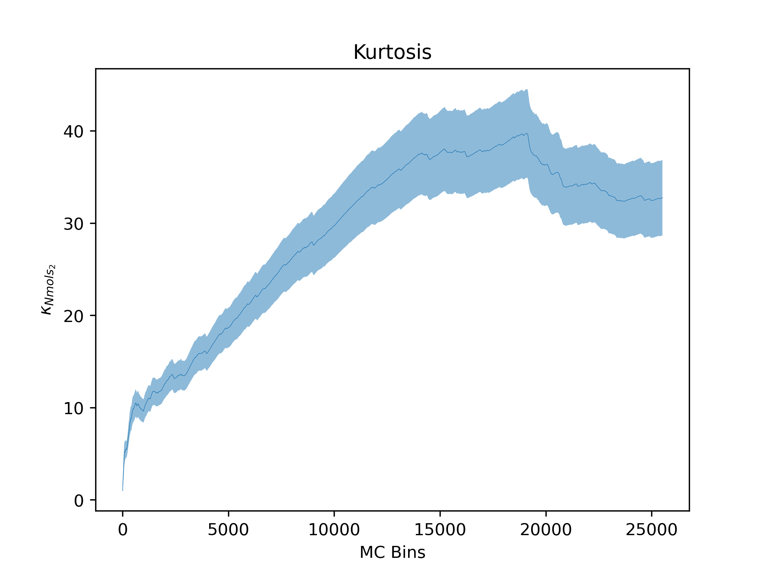
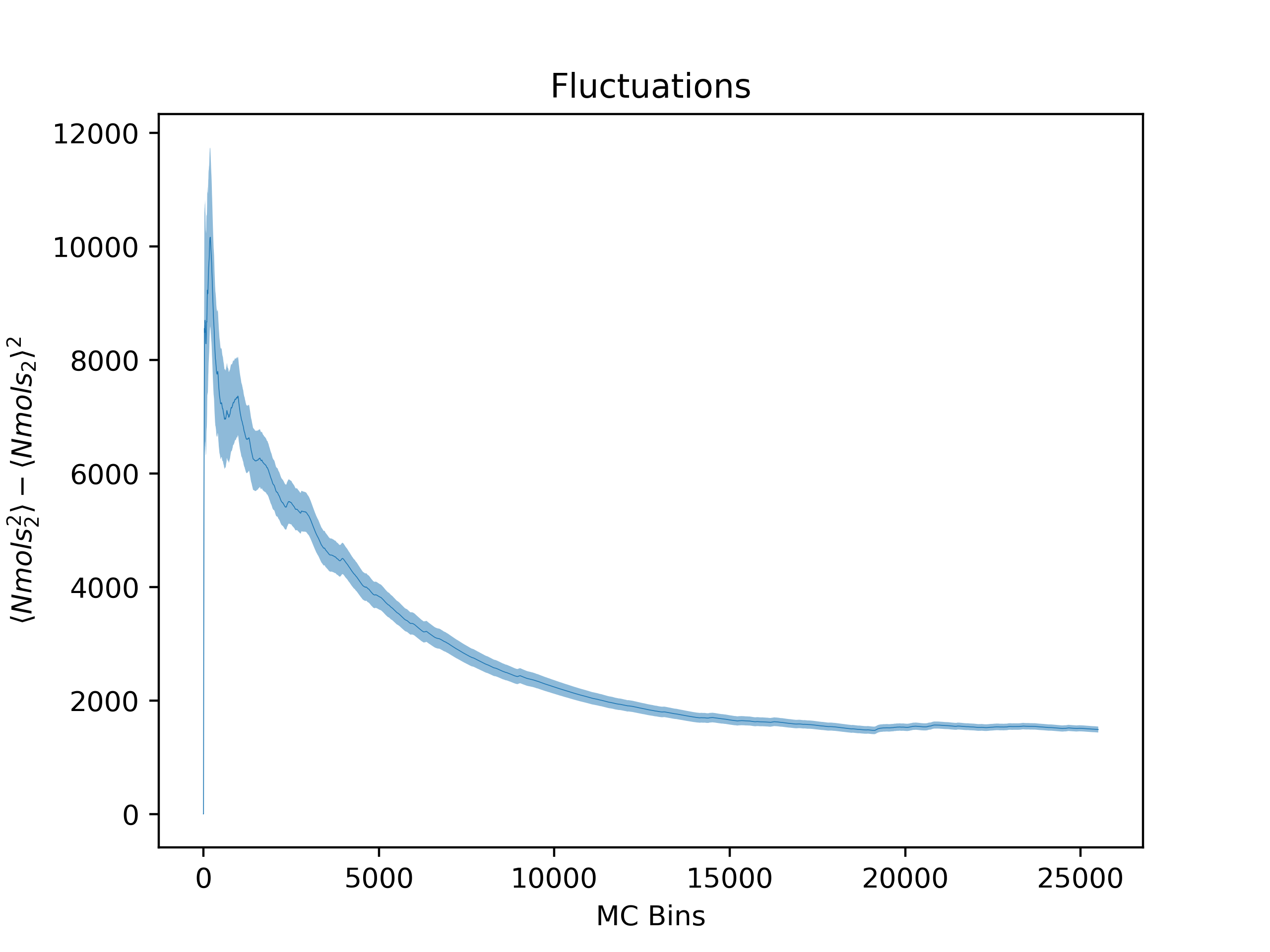
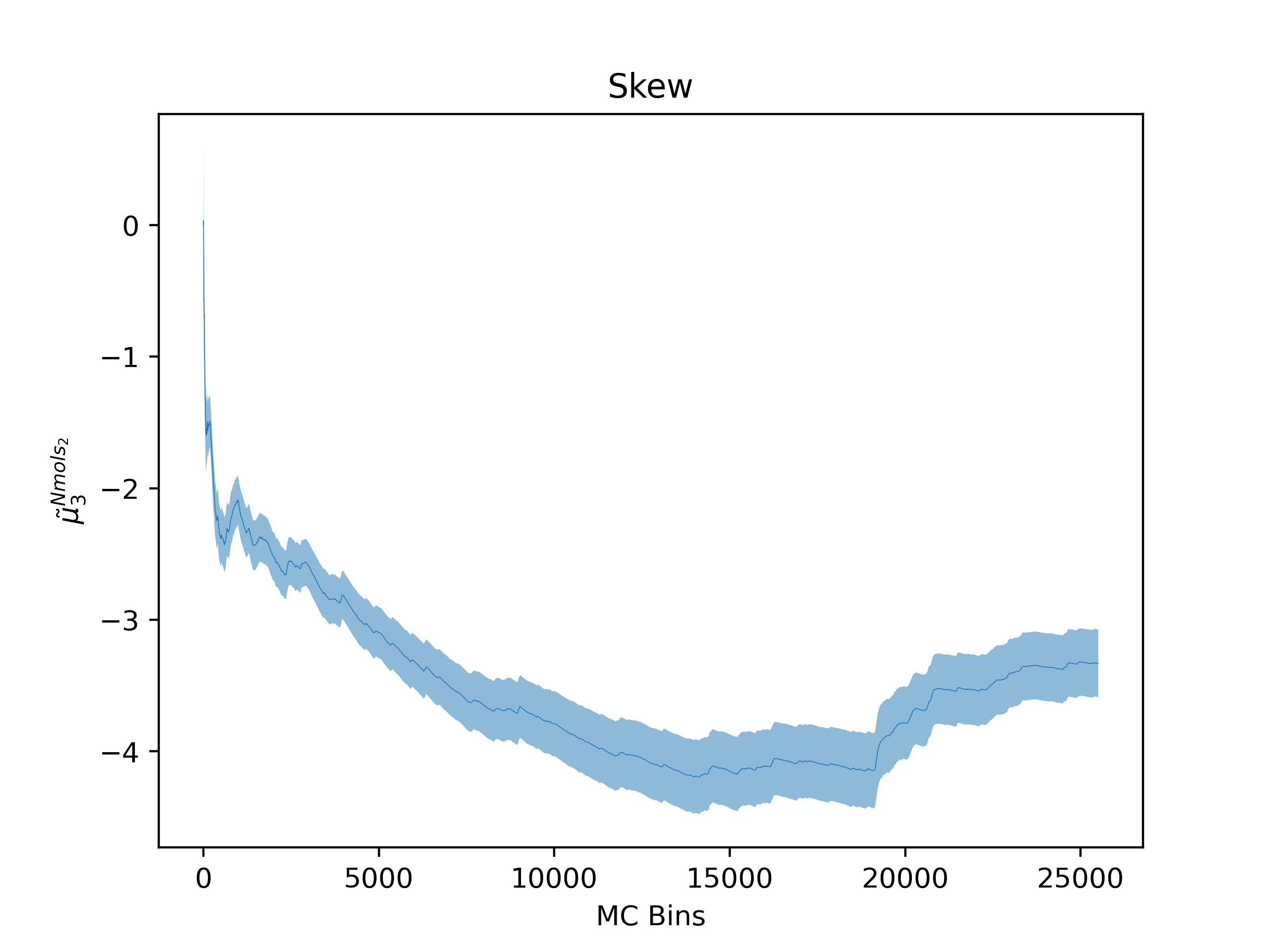
Command line methods have been included for convenience. Average, fluctuations, skew, and kurtosis can be plotted as a function of Monte Carlo step (or average bin) with errorbars. Binning analysis can also be performed. For the full set of options see
```
python -m erroranalysis --help
```
or
```
ea --help
```
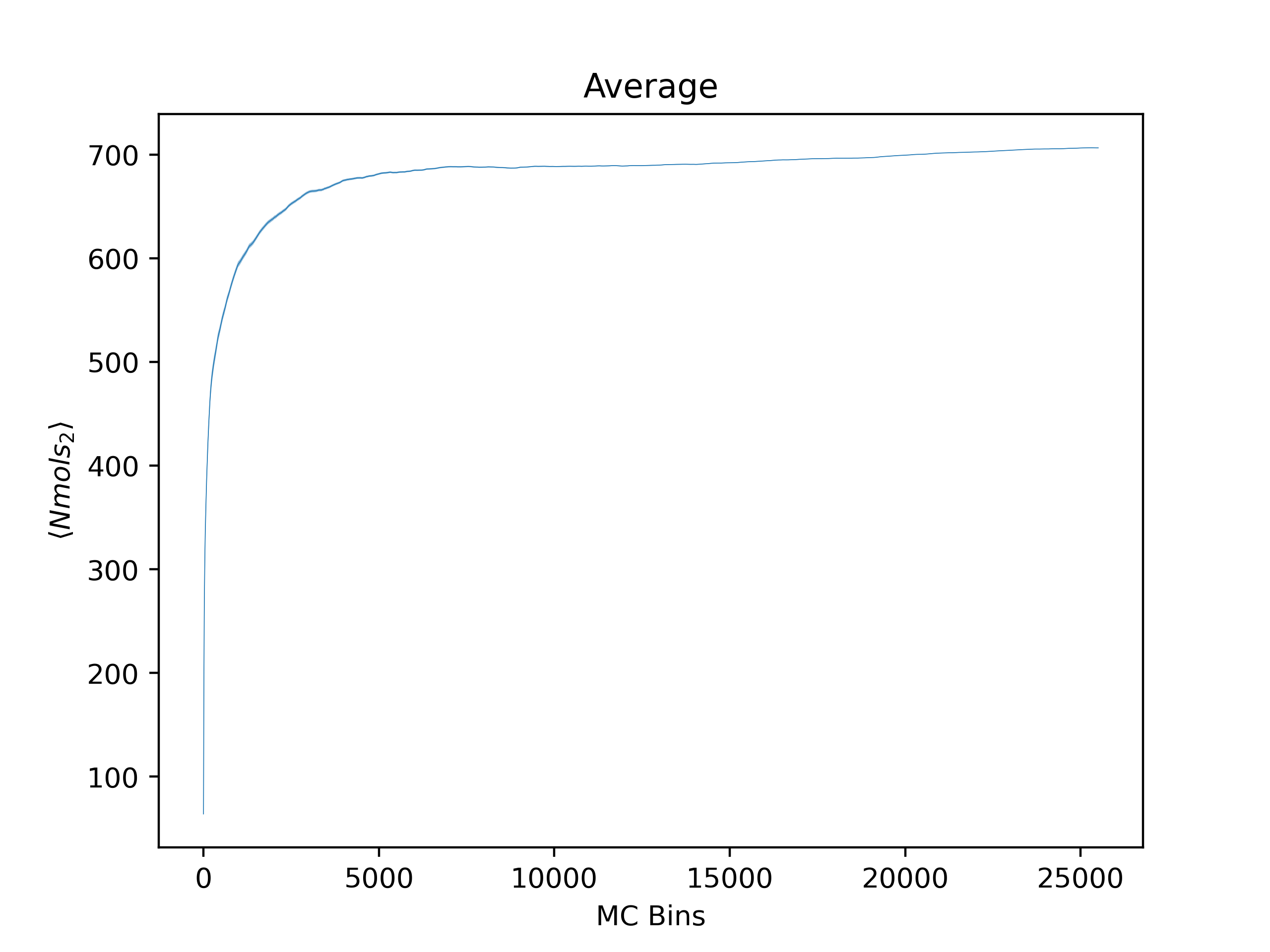
For example, the following command generates plots for the `Nmols_2` estimator (average number of particles):
```
ea --skip_header 1 --estimator Nmols_2 --savefig argon_MCM41_-12.68.png examples/argon_MCM41_-12.68.out.prp
```
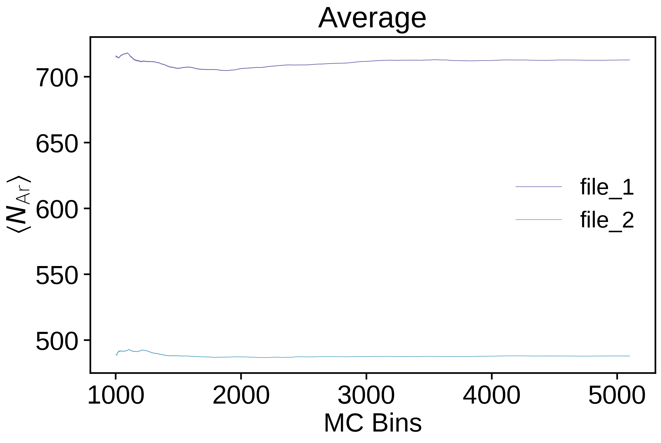
Note that Error Analysis will attempt to read the headers for each column of data in the data files provided and the estimator of interest should be specified from the header. In the example, the header for the data is on the second line so `--skip_header 1` is specified to skip the first line of the data file before attempting to read the header. A custom header can be provided if the header is missing on the datafiles and multiple data files are supported as well. Here several options are shown off:
```
ea --skip 5000 --bin_size 5 --skip_header 1 --custom_header "estimator_1,estimator_2,estimator_3,estimator_4,estimator_5" --estimator estimator_4 --pretty_estimator_name "N_\mathrm{Ar}" --savefig two_files_at_once.png --labels "file_1,file_2" --legend examples/argon_MCM41_-12.68.out.prp examples/argon_MCM41_-13.34.out.prp
```
Binning analysis can be performed by adding the `--binning_analysis` flag:
```
ea --skip 15000 --skip_header 1 --estimator Nmols_2 --binning_analysis --savefig argon_MCM41_-12.68.png examples/argon_MCM41_-12.68.out.prp
```
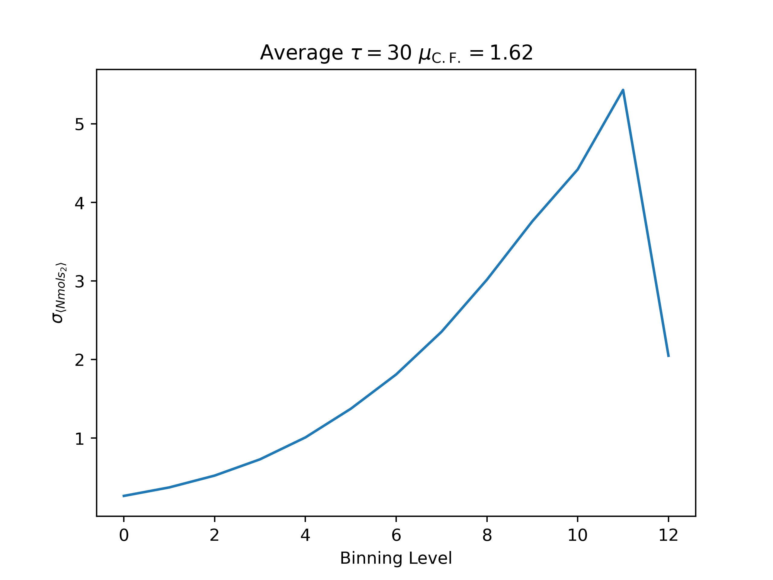
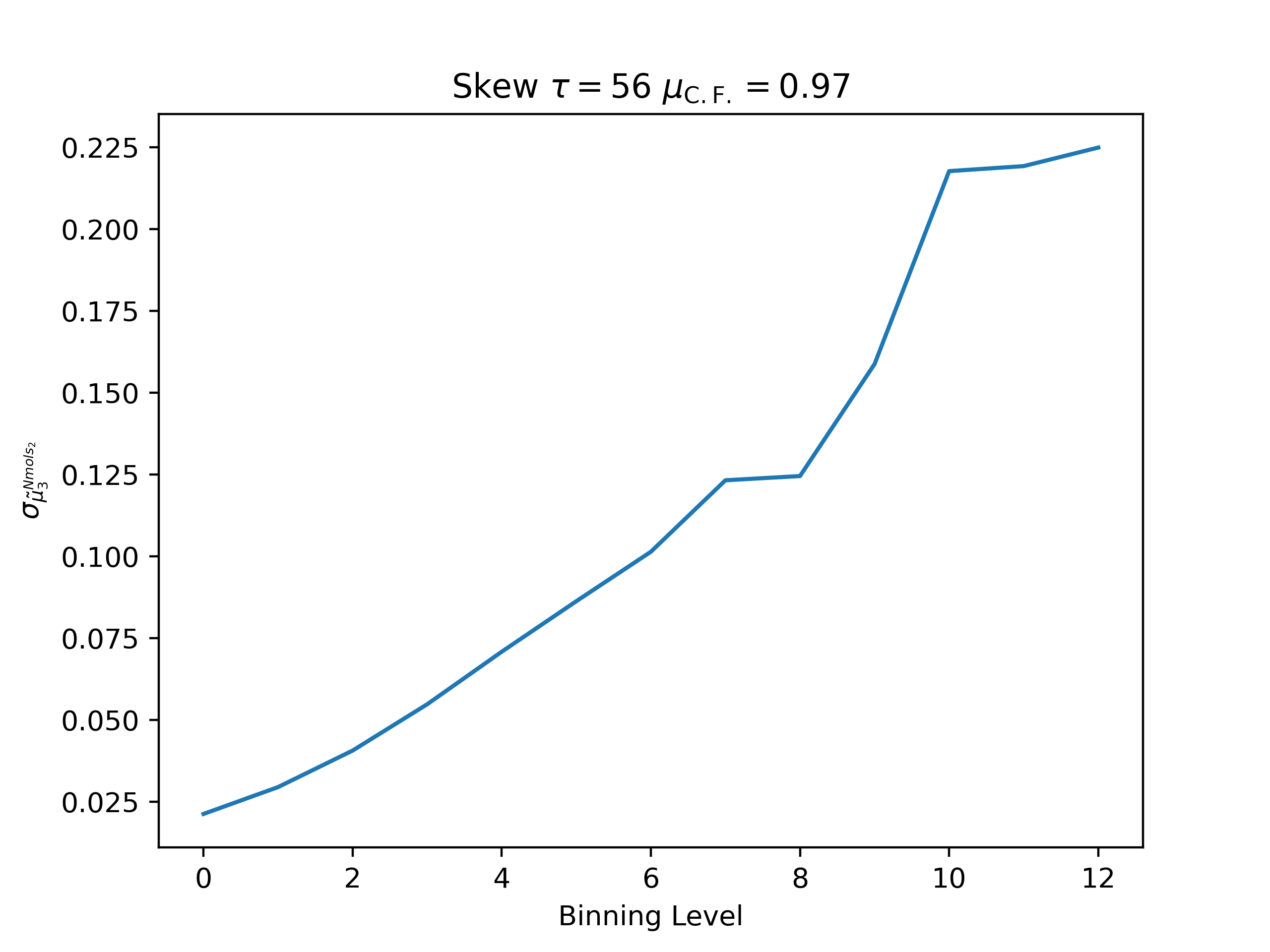
```
Average
autocorrelation time: 29.3695548682474
convergence factor: 1.6227794947682683
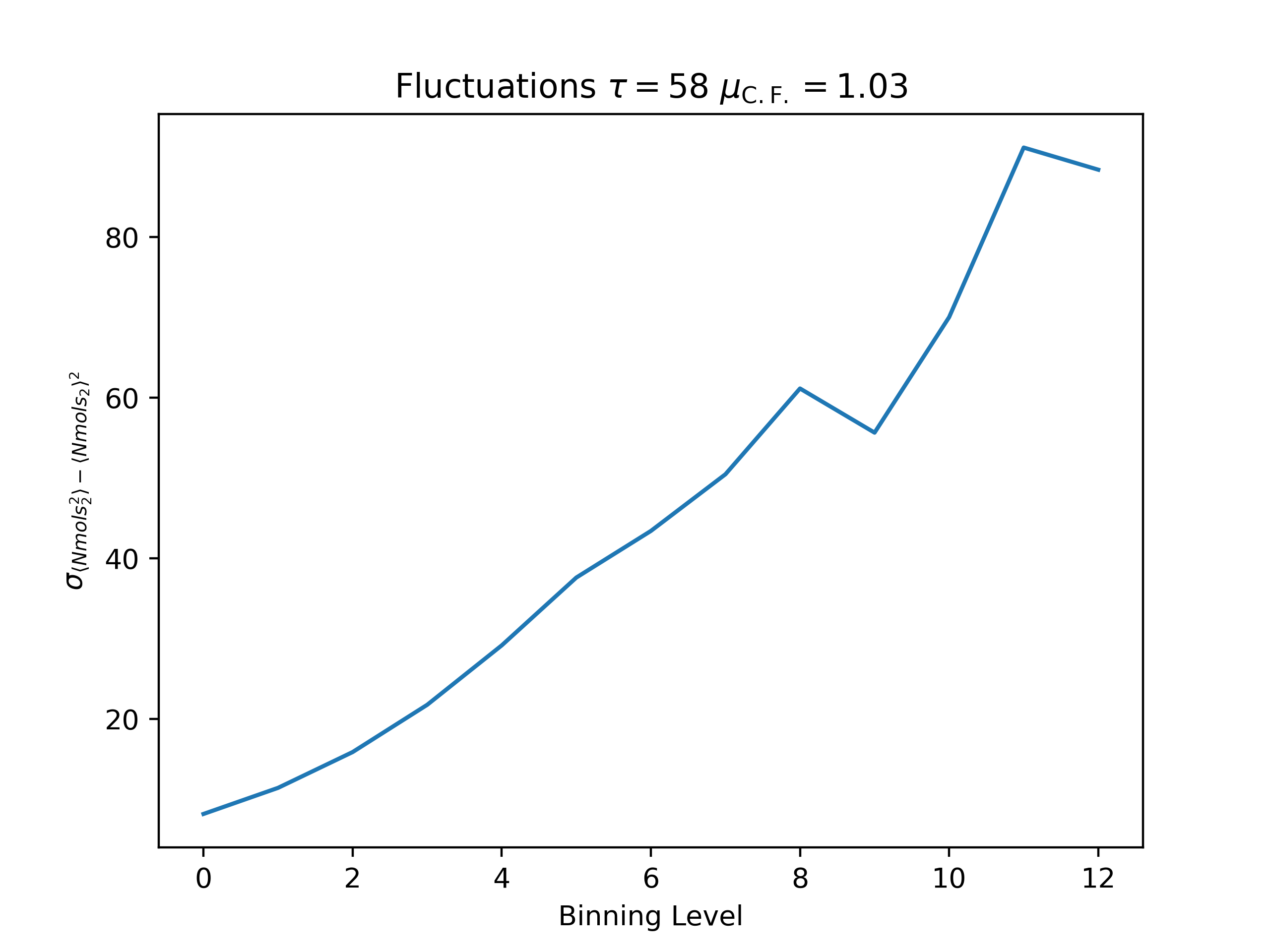
Fluctuations
autocorrelation time: 57.78295684564631
convergence factor: 1.0302306748178092
Skew
autocorrelation time: 55.363864907469626
convergence factor: 0.9741542111868422
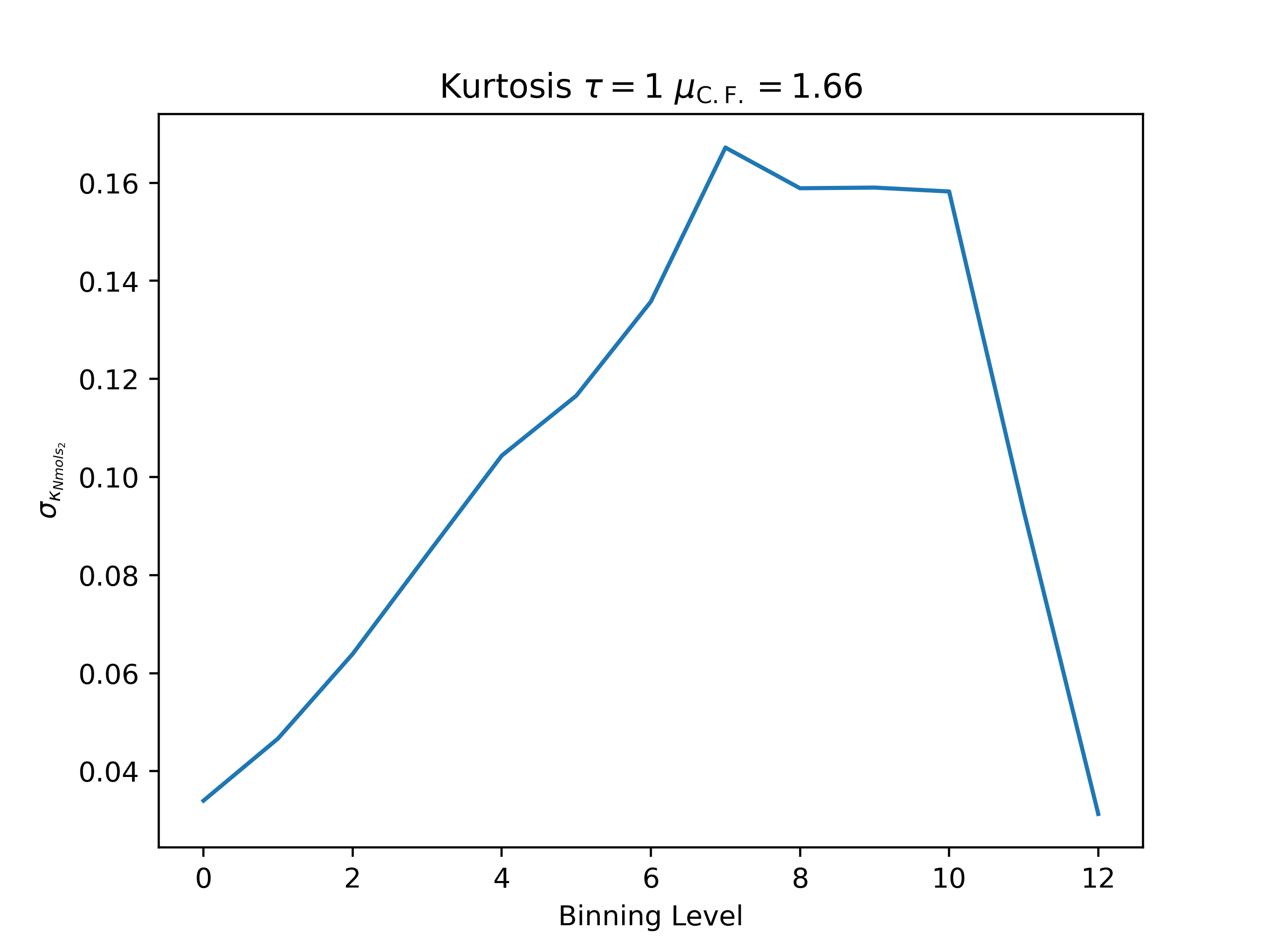
Kurtosis
autocorrelation time: -0.07655265212193901
convergence factor: 1.6641092137649522
```
## Advanced usage
More advanced usage of the Error Analysis package can be achieved by importing the pacakge directly into your project or notebook environment using `import erroranalysis as ea`. Some advanced usage cases are discussed below.
<a id='lattice_vectors'></a>
### Compressibility
The compressibility may be a measure of interest and can be calculated by
<img src="https://render.githubusercontent.com/render/math?math=%5CHuge%20%5Ckappa_T%20%3D%20%5Cfrac%7B1%7D%7B%5Crho_0%20k_%5Cmathrm%7BB%7D%20T%7D%5Cfrac%7B%5Clangle%20N%5E2%5Crangle%20-%20%5Clangle%20N%5Crangle%5E2%7D%7B%5Clangle%20N%5Crangle%7D">
where <img src="https://render.githubusercontent.com/render/math?math=%5Crho_0%20%3D%20%5Cfrac%7B%5Clangle%20N%5Crangle%7D%7BV%7D">
is the average particle density. Notice the compressibility is a function of averages. Jackknife or bootstrap resampling of the data may give a better measure of the error in the compressibility. Start with the compressibility as a function:
```python
def compressibility(N,N2,volume=1.0,k_B=1.0,T=1.0):
pf = volume/(k_B*T)
return pf*(((N2 - (N**2)))/(N**2))
```
Then use Error Analysis to calculate the average compressibility and error
```python
import erroranalysis as ea
import numpy as np
from scipy.constants import k as k_b
skip = 6000 # Skip some measurements
# Values specific to the argon in MCM-41 GCMC simulations
box_volume = 139357.3925 #\AA^3
volume = box_volume*((1e-10)**3)
temperature = 87.35 #K
# Load the GCMC data
fn = "examples/argon_MCM41_-12.68.out.prp"
_data = np.genfromtxt(fn,names=True,skip_header=1)
#Calculate average compressibility and error using jackknife method
κ_avg, κ_err = ea.jackknife_on_function( compressibility,
_data["Nmols_2"][skip:],
_data["Nmols_2"][skip:]**2,
volume=volume,
k_B=k_b,
T=temperature)
print("κ_avg = {:.5e}".format(κ_avg))
print("κ_err = {:.5e}".format(κ_err))
```
κ_avg = 1.65368e-07
κ_err = 1.53513e-09
Notice we pass the `compressibility()` function as the first argument to the `jackknife_on_function()` and then the arguments to `compressibility()` (including keyword arguments). Bootstrap sampling can similarly be performed using `bootstrap_on_function()`. These methods are used when generating the fluctuations, skew, and kurtosis.
## Additional usage
The functions `jackknife()`, `bootstrap()`, `jackknife_on_function()`, and `boostrap_on_function()` operate on array-like data. See the documentation to discover more creative usage!


