# DSPFTW
Starting points and helper functions for learning digital signal processing.
## Setup
If you haven't already, install Python 3.5 or greater, and the `dspftw` package.
```sh
python3 -m pip install dspftw --user
```
## Intro
### Decomposition
[Superposition: The foundation of DSP](http://www.dspguide.com/ch5/6.htm)
### Sinusoids
Prefer to use the complex exponential form instead of real, as it's a more natural fit for fourier analysis and synthesis.
The following functions represent a complex sinusoid. They are equivalent, and take the same parameters:
* A = Amplitude (y axis is amplitude).
* f = Frequency (cycles per second) in Hertz. It is multiplied by 2π to get radians per second.
* t = Time in seconds. These functions work in the time domain (x axis is time).
* ϕ = Phase offset at t=0, in radians.
```
z(t) = A*exp(j*(2π*f*t+ϕ))
z(t) = A*cos(2π*f*t+ϕ)+j*A*sin(2π*f*t+ϕ)
```
We can define this in Python with the following.
```python
import numpy as np
# Here we use the name "complex_sinusoid" instead of just "z".
def complex_sinusoid(A, f, t, phi): return A * np.exp(1j*(2*np.pi*f*t+phi))
```
In fact, this is defined in the `dspftw` package, so let's import that.
```python
import dspftw
```
We can create our own sinusoid by defining everything except `t`.
```python
def my_sinusoid(t): return dspftw.complex_sinusoid(A=5, f=5, t=t, phi=0)
```
We can get the signal at a bunch of times thanks to numpy arrays. We use `numpy.linspace` to generate the evenly spaced times.
```python
import numpy as np
times = np.linspace(0, 1, num=25) # 25 evenly spaced values between 0 and 1
my_signal = my_sinusoid(times) # returns an array of complex values representing the signal
```
Now plot it out with `dspftw.plot_complex()`, which uses matplotlib.
```python
import matplotlib.pyplot as plt
dspftw.plot_complex(my_signal)
plt.show()
```
[Complex Exponential Signals](https://www.cs.ccu.edu.tw/~wtchu/courses/2012s_DSP/Lectures/Lecture%203%20Complex%20Exponential%20Signals.pdf)
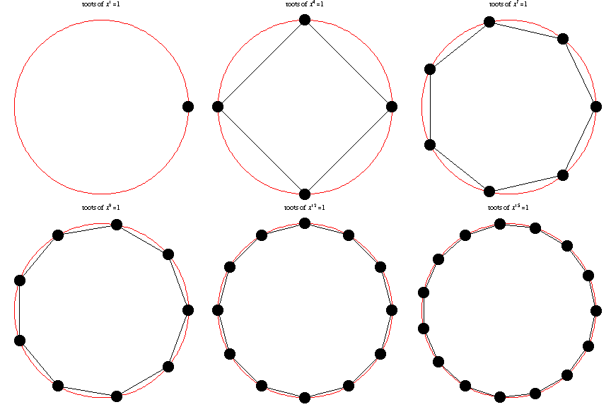
### Roots of Unity

[Wolfram Mathworld](https://mathworld.wolfram.com/RootofUnity.html)
### Delta Function
### Conjugate
[Complex Conjugate](https://en.wikipedia.org/wiki/Complex_conjugate)
### Convolution
[Convolution](https://www.dspguide.com/ch6/2.htm)
### Correlation
[numpy.correlate](https://numpy.org/doc/stable/reference/generated/numpy.correlate.html)
### Kronecker Product
[numpy.kron](https://numpy.org/doc/stable/reference/generated/numpy.kron.html)
### Sample Signals
[SigIDWiki sample signals](https://www.sigidwiki.com/)
### Loading Signals
#### Complex 8 bit
```python
import numpy as np
signal = np.fromfile('filename', dtype='b') # load the whole file
signal = np.fromfile('filename', dtype='b', count=1024) # only load the first 1024 bytes of the file
signal = np.fromfile('filename', dtype='b', offset=1024) # skip the first 1024 bytes of the file
signal = np.fromfile('filename', dtype='b', offset=1024, count=1024) # skip 1024, then load 1024
```
This just loads the values as an array of real numbers, but we want it as complex. We have to interpret every other value as the imaginary component.
```python
signal = signal[0::2] + signal[1::2]*1j
```
#### Complex 32 bit float, little-endian (x86)
```python
signal = np.fromfile('filename', dtype='<f')
```
`count` and `offset` work as above, but note that `offset` is in bytes, so you must multiple by 4 since there are 4 bytes in 32 bits.
#### Complex 32 bit float, big-endian
```python
signal = np.fromfile('filename', dtype='>f')
```
`count` and `offset` work as above, but note that `offset` is in bytes, so you must multiple by 4 since there are 4 bytes in 32 bits.


