# compressnets
Compressnets is a Python package designed to compress high-resolution temporal network data (eg. contact networks)
to lower resolution, while maintaining important temporal structural features.
Compressnets is designed for taking sequences of static networks (represented as adjacency matrices)
and compressing them to a user-specified reduced number of adjacency matrices. For example, say you
have contact data at the resolution of 20 seconds, over the course of 24 hours, which can be represented
as 4,320 adjacency matrices.
You might wish to compress the data from the original 4,320 adjacency matrices into the best 20 adjacency matrices
that best represent the temporal dynamics. The
`compressnets` package can help you to progressively aggregate the data into the best 20 representative "snapshots"
(single static network valid for a duration of time).
Pre-print with further details on the compression algorithm and theoretical framework is available [on the arXiv](https://arxiv.org/abs/2205.11566).
## Most basic usage
This example is just to show how to use the package. In practice, 3 starting snapshots is unrealistic as there wouldn't
be a need to use an algorithm for compressing 3 snapshots into 2, so this example just demonstrates package usage in a simple way.
See below for a usage demo using a built-in sample network.
To use `compressnets`, install the package via the PyPi index via
`pip install compressnets`.
The core elements of `compressnets` are the objects, `network.TemporalNetwork` and `network.Snapshot`,
and the algorithm `compression.Compressor.compress(...)`.
Follow along the following example in your own Python workspace with
```
from compressnets import compression, network
```
As an example, create NumPy arrays to represent your adjacency matrices (or load them from data via your own code):
```
matrix_1 = np.array([[0, 0, 1],[0, 0, 1],[1, 1, 0]])
matrix_2 = np.array([[0, 1, 1],[1, 0, 1],[1, 1, 0]])
matrix_3 = np.array([[0, 1, 0],[1, 0, 1],[0, 1, 0]])
```
Next, you will be creating `Snapshot` objects out of your arrays. A snapshot is simply an adjacency matrix
coupled with a start time, end time, and `beta` value, which will be used in the computation process for the
compression algorithm.
#### Note: While the durations of each snapshot may vary in length from one another, the `end_time` of one snapshot should be the `start_time` of the next one. In other words, there should not be gaps in your snapshots.
#### Note: It's also best practice to set the very first `start_time` as 0. The `to_snapshot_list()` helper function will do this automatically, but if you configure snapshots by hand, be sure to standardize to start at 0.
If the duration of all of your snapshots is uniform, you can use the `TemporalData` object
as a helper object to quickly make a series of snapshots using your list of adjacency matrices, like this:
```
infect_rate = 0.5
your_temporal_data = network.TemporalData([matrix_1, matrix_2, matrix_3], interval=1, beta=infect_rate)
snapshots = your_temporal_data.to_snapshot_list()
```
See section below on choosing `beta`, but for this example, it can be any value between 0 and 1.
#### Note: `beta` should be the same for all snapshots in the list.
If your snapshots have custom durations and are not all equal to the same interval, you can instead
create your own list of `Snapshot` objects from your arrays, equipped with a consecutive start and end time for each,
(instead of using the `TemporalData` helper):
```
snapshots = [network.Snapshot(start_time=0, end_time=1, beta=infect_rate, A=matrix_1),
network.Snapshot(start_time=1, end_time=2, beta=infect_rate, A=matrix_2),
network.Snapshot(start_time=2, end_time=3, beta=infect_rate, A=matrix_3)]
```
Either way, once you have a list of `Snapshot` objects,
then create a `TemporalNetwork` object to contain all of your ordered snapshots:
```
your_temporal_network = network.TemporalNetwork(snapshots)
```
Using the algorithmic compression from our paper [link], you can compress
the temporal network into a desired number of compressed snapshots (in this example, 2), by calling on an instance of
the static `Compressor` class
```
your_compressed_network_result = compression.Compressor.compress(your_temporal_network,
compress_to=2,
how='optimal')
```
which will return the new `TemporalNetwork` object, and also the total induced error from the snapshots that
were selected for compression. The elements can be accessed via a dictionary as
```
your_compressed_network = your_compressed_network_result["compressed_network"]
total_induced_error = your_compressed_network_result["error"]
```
To compress your original network into an even division and aggregation of snapshots,
not using our algorithm, you can call `compress` and changing the `how` argument to `even`:
```
your_even_compressed_network_result = compression.Compressor.compress(your_temporal_network,
compress_to=2,
how='even')
even_compressed_network = your_even_compressed_network_result["compressed_network"]
```
From the resulting compressed `TemporalNetwork` objects, you can now access your snapshots as you
would with your original temporal network, by accessing the `snapshots` member via
```
your_new_snapshots = your_compressed_network.snapshots
```
from which you can access each snapshot's new duration, adjacency matrix, start and end times.
## Usage using demo network
For a more involved demo, make use of the `compressnets.demos` module to access a more complex
temporal network without having to create one yourself. Follow the code below in your
own workspace to use a sample temporal network to compress it, and visualize a system of ODEs over
the compressed network vs. the original temporal solution.
```
from compressnets import compression, network, demos, solvers
demo_network = demos.Sample.get_sample_temporal_network()
compressed_optimal = compression.Compressor.compress(demo_network, compress_to=4, how='optimal')["compressed_network"]
compressed_even = compression.Compressor.compress(demo_network, compress_to=4, how='even')["compressed_network"]
```
Now you have the resulting compressed temporal networks for the optimal (algorithmic) method and from an even
aggregation method.
To visualize the new time boundaries of each aggregated snapshot, and compare a full
Susceptible-Infected disease spread process against the fully temporal network, you can
utilize the `compressnets.solvers` module to solve a system of ODEs and plot the resulting figure:
```
## Creating and solving a model with the original temporal network
N = demo_network.snapshots[0].N
beta = demo_network.snapshots[0].beta
model = solvers.TemporalSIModel({'beta': beta}, np.array([1/N for _ in range(N)]),
demo_network.snapshots[demo_network.length-1].end_time,
demo_network)
soln = model.solve_model()
smooth_soln = model.smooth_solution(soln)
plt.plot(smooth_soln[0], smooth_soln[1], color='k', label='Temporal solution')
plt.vlines(list(demo_network.get_time_network_map().keys()), ymin=0, ymax=N/3, ls='-',
lw=0.5, alpha=1.0, color='k')
## Creating and solving a model with the algorithmically compressed temporal network
N = compressed_optimal.snapshots[0].N
beta = compressed_optimal.snapshots[0].beta
model = solvers.TemporalSIModel({'beta': beta}, np.array([1/N for _ in range(N)]),
compressed_optimal.snapshots[compressed_optimal.length-1].end_time,
compressed_optimal)
soln = model.solve_model()
smooth_soln = model.smooth_solution(soln)
plt.plot(smooth_soln[0], smooth_soln[1], color='b', label='Optimal compressed')
plt.vlines(list(compressed_optimal.get_time_network_map().keys()), ymin=N/3, ymax=2*N/3, ls='-',
lw=0.5, alpha=1.0, color='b')
## Creating and solving a model with the evenly compressed temporal network
N = compressed_even.snapshots[0].N
beta = compressed_even.snapshots[0].beta
model = solvers.TemporalSIModel({'beta': beta}, np.array([1/N for _ in range(N)]),
compressed_even.snapshots[compressed_even.length-1].end_time,
compressed_even)
soln = model.solve_model()
smooth_soln = model.smooth_solution(soln)
plt.plot(smooth_soln[0], smooth_soln[1], color='r', label='Even compressed')
plt.vlines(list(compressed_even.get_time_network_map().keys()), ymin=2*N/3, ymax=N, ls='-',
lw=0.5, alpha=1.0, color='r')
plt.ylabel('Number infected')
plt.xlabel('Time')
plt.legend()
plt.show()
```
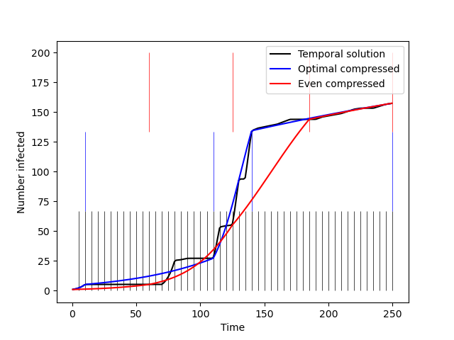
Output figure from the sample code above using the provided demo temporal network.
The original temporal network has 50 snapshots and is compressed down to 4 snapshots.
In blue, you see the resulting temporal boundaries of the 4 snapshots compressed using our
algorithm. In red, you see the resulting temporal boundaries of the 4 snapshots compressed
into even-size aggregate matrices. The time series represent an SI epidemic process over the
3 versions of the network.
## Choosing the infect rate `beta`
The best `beta` value to choose for your series of networks is one that,
given an SI process over the full sequence of temporal networks,
won't saturate (infect the entire network) too quickly, but that also provides
rich enough dynamics that can be observed.
One way to test if a given `beta` value is appropriate is to use the `solvers` module.
The same module that is shown in the demo to assess how your compression
performed is also just as useful for a pre-analysis of your system.
For example, running just the top block of the demo above will give you a time series solution
on your full temporal network:
```
N = demo_network.snapshots[0].N
beta = YOUR_CHOSEN_VALUE
model = solvers.TemporalSIModel({'beta': beta}, np.array([1/N for _ in range(N)]),
demo_network.snapshots[demo_network.length-1].end_time,
demo_network)
soln = model.solve_model()
smooth_soln = model.smooth_solution(soln)
plt.plot(smooth_soln[0], smooth_soln[1], color='k', label='Temporal solution')
```
You can try out a range of different `beta` values until you see a time series
solution that doesn't saturate too quickly and also doesn't die off.
The compression algorithm is robust to a range of values around your specified value,
so no need to worry about a precise value of `beta`, just one that's in the appropriate range
for the epidemic dynamics to be observed.
## Citation
If you use this package, please name your use of this package as well as the original
paper on the framework, as
Allen, Andrea J. and Moore, Cristopher and Hébert-Dufresne, Laurent.
A network compression approach for quantifying the importance of temporal contact chronology.
Preprint at https://arxiv.org/abs/2205.11566 (2022).
Code written and maintained by Andrea Allen.


