<h1> <img style="height:5em;" alt="batty" src="https://raw.githubusercontent.com/philippeller/batty/main/batty_logo.svg"/> </h1>
# BAT to Python (batty)
A small python interface to the Bayesian Analysis Toolkit (BAT.jl) https://github.com/bat/BAT.jl
* Please check out the minimal example to get started [below](#minimal-example)
* To understand how to define a prior + likelihood, please read [this](#specifying-priors-and-likelihoods)
* For experimental support of gradients, see [this](#hmc-with-gradients)
# Quick Start
## Installation
There are two parts to an installation, one concerning the python side, and one the julia side:
* Python: `pip install batty`
* Julia: `import Pkg; Pkg.add.(["PyJulia", "DensityInterface", "Distributions", "ValueShapes", "TypedTables", "ArraysOfArrays", "ChainRulesCore", "BAT"])`
## Minimal Example
The code below is showing a minimal example:
* using a gaussian likelihood and a uniform prior
* generating samples via Metropolis-Hastings
* plotting the resulting sampes
* <s>estimating the integral value via BridgeSampling</s>
```python
%load_ext autoreload
%autoreload 2
```
```python
import numpy as np
import matplotlib.pyplot as plt
%matplotlib inline
from batty import BAT_sampler, BAT, Distributions, jl
```
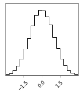
```python
sampler = BAT_sampler(llh=lambda x : -0.5 * x**2, prior_specs=Distributions.Uniform(-3, 3))
sampler.sample();
sampler.corner();
```
# Usage
## Using Different Algotihms
There are a range of algorihtms available within BAT, and those can be further customized via arguments. Here are just a few examples:
### MCMC Sampling:
```python
results = {}
```
* Metropolis-Hastings:
```python
results['Metropolis-Hastings'] = sampler.sample(strategy=BAT.MCMCSampling(nsteps=10_000, nchains=2))
```
* Metropolis-Hastings with Accept-Reject weighting:
```python
results['Accept-Reject Weighting'] = sampler.sample(strategy=BAT.MCMCSampling(mcalg=BAT.MetropolisHastings(weighting=BAT.ARPWeighting()), nsteps=10_000, nchains=2))
```
* Prior Importance Sampling:
```python
results['Prior Importance Sampling'] = sampler.sample(strategy=BAT.PriorImportanceSampler(nsamples=10_000))
```
* Sobol Sampler:
```python
results['Sobol Quasi Random Numbers'] = sampler.sample(strategy=BAT.SobolSampler(nsamples=10_000))
```
* Grid Sampler:
```python
results['Grid Points'] = sampler.sample(strategy=BAT.GridSampler(ppa=1000))
```
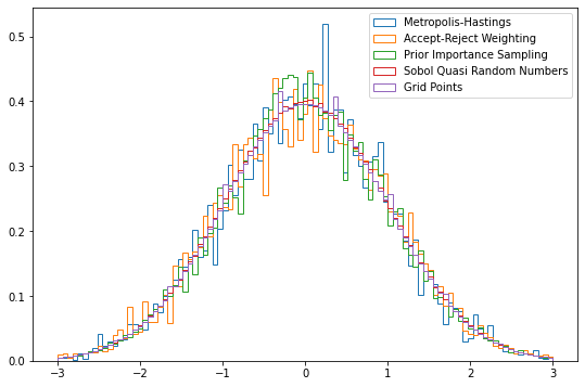
Plotting the different results:
```python
fig = plt.figure(figsize=(9,6))
bins=np.linspace(-3, 3, 100)
for key, item in results.items():
plt.hist(item.v, weights=item.weight, bins=bins, density=True, histtype="step", label=key);
plt.legend()
```
<matplotlib.legend.Legend at 0x7f069fcd5ee0>
# Specifying Priors and Likelihoods
Priors are specified via Julia `Distributions`, multiple Dimensions can be defined via a `dict`, where the `key` is the dimension name and the value the distribution, or as a list in case flat vectors with paraeter names are used.
Below the example *with* parameter names
```python
s = np.array([[0.25, 0.4], [0.9, 0.75]])
prior_specs = {'a' : Distributions.Uniform(-3,3), 'b' : Distributions.MvNormal(np.array([1.,1.]), jl.Array(s@s.T))}
```
The log-likelihood (`llh`) can be any python callable, that returns the log-likelihood values. The first argument to the function is the object with paramneter values, here `x`. If the prior is simple (i.e. like in the example in the beginning, `x` is directly the parameter value). If the prior is specified via a `dict`, then `x` contains a field per parameter with the value.
Any additional `args` to the llh can be given in the sampler, such as here `d` for data:
```python
def llh(x, d):
return -0.5 * ((x.b[0] - d[0])**2 + (x.b[1] - d[1])**2/4) - x.a
```
Or alternatively *without* parameter names (this will result in a flat vector):
```python
# prior_specs = [Distributions.Uniform(-3,3), Distributions.MvNormal(np.array([1.,1.]), jl.Array(s@s.T))]
# def llh(x, d):
# return -0.5 * ((x[1] - d[0])**2 + (x[2] - d[1])**2/4) - x[0]
```
```python
d = [-1, 1]
```
```python
sampler = BAT_sampler(llh=llh, prior_specs=prior_specs, llh_args=(d,))
```
Let us generate a few samples:
```python
sampler.sample(strategy=BAT.MCMCSampling(nsteps=10_000, nchains=2));
```
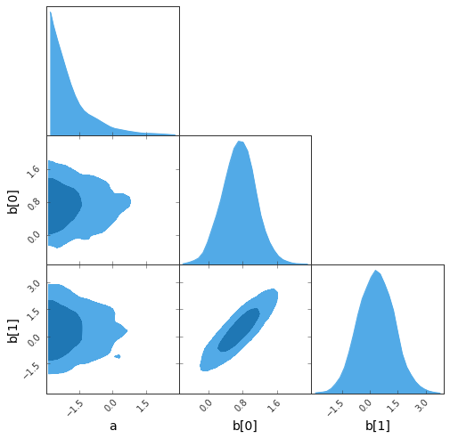
### Some interface to plotting tools are available
* The **G**reat **T**riangular **C**onfusion (GTC) plot:
```python
sampler.gtc(figureSize=8, customLabelFont={'size':14}, customTickFont={'size':10});
```
findfont: Font family ['Arial'] not found. Falling back to DejaVu Sans.
findfont: Font family ['Arial'] not found. Falling back to DejaVu Sans.
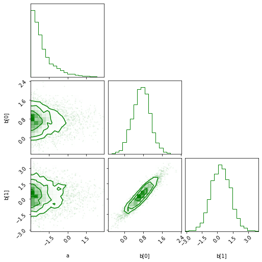
* The corner plot:
```python
sampler.corner(color='green');
```
## HMC with Gradients
This at the moment only works with preiors defined as flat vectors!
```python
llh = lambda x : -0.5 * np.dot(x, x)
grad = lambda x : -x
sampler = BAT_sampler(llh=llh, prior_specs=[Distributions.Uniform(-3, 3),], grad=grad, )
# Or alternatively:
# llh_and_grad = lambda x: (-0.5 * np.dot(x, x), -x)
# sampler = BAT_sampler(llh=llh, prior_specs=[Distributions.Uniform(-3, 3),], llh_and_grad=llh_and_grad)
sampler.sample(strategy=BAT.MCMCSampling(mcalg=BAT.HamiltonianMC()));
sampler.corner();
```

```python
```


