baggingrnet: Library for Bagging of Deep Residual Neural Networks
================
### Introduction
This package provides The python Library for Bagging of Deep Residual Neural Networks (baggingrnet). Current version just supports the KERAS package of deep learning and will extend to the others in the future. The following functionaity is provoded in this package: \* model multBagging: Major class to parallel bagging of autoencoder-based deep residual networks. You can setup its aruments for optimal effects. See the class and its member functions' help for details.
resAutoencoder: Major class of the base model of autoencoder-based deep residual network. See the specifics for its details. ensPrediction: Major class to ensemble predictions and optional evaluation for independent test.
\* util pmetrics: main metrics including rsquare and rmse etc.
- data data: function to access two sample datas to test and demonstrate parallel training and predictions of multiple models by bagging. simData: function to simulate the dataset for a test.
### Installation of the package
1. You can directly install this package using the following command for the latest version:
pip install baggingrnet
2. You can also clone the repository and then install:
git clone --recursive https://github.com/lspatial/baggingrnet.git
pip install ./setup.py install
### Modeling Framework
The modeling is based on bagging of the encoding-decoding antoencoder based deep residual multilayer percepton (MLP). Residual connections were used from the encoding to decoding layers to improve the learning efficiency and use of bagging is to achieve the stable and improved ensemble predictions, with uncertainty metric (standard deviation). <img align="center" src="https://raw.githubusercontent.com/lspatial/baggingrnet/master/figs/framework.jpg" style="zoom:50%" hspace="2"/>
The relevant paper will be published and will update here once published.
### Example 1: Regression of Simulated Data
The dataset is simulated using the following formula: <img align="center" src="https://raw.githubusercontent.com/lspatial/baggingrnet/master/figs/simform.png" hspace="2"/>
each covariate defined as:
*x*<sub>1</sub> ∼ *U*(1, 100),*x*<sub>2</sub> ∼ *U*(0, 100),*x*<sub>3</sub> ∼ *U*(1, 10),*x*<sub>4</sub> ∼ *U*(1, 100),*x*<sub>5</sub> ∼ *U*(9, 100),*x*<sub>6</sub> ∼ *U*(1, 1009),*x*<sub>7</sub> ∼ *U*(5, 300),*x*<sub>8</sub> *U*(6 ∼ 200)
This example is to illustrate how to use bagging class to train a model and compare the results by the models with and without use of residual connections in the models.
###### 1) Load the dataset:
``` python
from baggingrnet.data import data
sim_train=data('sim_train')
sim_train['gindex']=np.array([i for i in range(sim_train.shape[0])])
```
``` r
knitr::kable(py$sim_train[c(1:5),], format = "html")
```
<table>
<thead>
<tr>
<th style="text-align:left;">
</th>
<th style="text-align:right;">
x1
</th>
<th style="text-align:right;">
x2
</th>
<th style="text-align:right;">
x3
</th>
<th style="text-align:right;">
x4
</th>
<th style="text-align:right;">
x5
</th>
<th style="text-align:right;">
x6
</th>
<th style="text-align:right;">
x7
</th>
<th style="text-align:right;">
x8
</th>
<th style="text-align:right;">
y
</th>
<th style="text-align:right;">
gindex
</th>
</tr>
</thead>
<tbody>
<tr>
<td style="text-align:left;">
9842
</td>
<td style="text-align:right;">
69.59893
</td>
<td style="text-align:right;">
6.368696
</td>
<td style="text-align:right;">
5.950720
</td>
<td style="text-align:right;">
97.97698
</td>
<td style="text-align:right;">
81.77670
</td>
<td style="text-align:right;">
38.12578
</td>
<td style="text-align:right;">
38.71023
</td>
<td style="text-align:right;">
124.90578
</td>
<td style="text-align:right;">
168.7697448
</td>
<td style="text-align:right;">
0
</td>
</tr>
<tr>
<td style="text-align:left;">
2513
</td>
<td style="text-align:right;">
88.83580
</td>
<td style="text-align:right;">
47.619385
</td>
<td style="text-align:right;">
8.107348
</td>
<td style="text-align:right;">
23.95389
</td>
<td style="text-align:right;">
41.00300
</td>
<td style="text-align:right;">
256.75319
</td>
<td style="text-align:right;">
203.75759
</td>
<td style="text-align:right;">
146.79040
</td>
<td style="text-align:right;">
184.8472212
</td>
<td style="text-align:right;">
1
</td>
</tr>
<tr>
<td style="text-align:left;">
9116
</td>
<td style="text-align:right;">
65.32664
</td>
<td style="text-align:right;">
49.473679
</td>
<td style="text-align:right;">
5.982418
</td>
<td style="text-align:right;">
75.99401
</td>
<td style="text-align:right;">
80.56275
</td>
<td style="text-align:right;">
849.48435
</td>
<td style="text-align:right;">
204.52137
</td>
<td style="text-align:right;">
161.61705
</td>
<td style="text-align:right;">
-444.5390646
</td>
<td style="text-align:right;">
2
</td>
</tr>
<tr>
<td style="text-align:left;">
2673
</td>
<td style="text-align:right;">
21.72827
</td>
<td style="text-align:right;">
64.946680
</td>
<td style="text-align:right;">
2.592348
</td>
<td style="text-align:right;">
70.32067
</td>
<td style="text-align:right;">
42.27824
</td>
<td style="text-align:right;">
387.42060
</td>
<td style="text-align:right;">
13.15852
</td>
<td style="text-align:right;">
88.47877
</td>
<td style="text-align:right;">
-166.3553631
</td>
<td style="text-align:right;">
3
</td>
</tr>
<tr>
<td style="text-align:left;">
5607
</td>
<td style="text-align:right;">
69.45317
</td>
<td style="text-align:right;">
18.811648
</td>
<td style="text-align:right;">
5.624373
</td>
<td style="text-align:right;">
39.81835
</td>
<td style="text-align:right;">
84.80446
</td>
<td style="text-align:right;">
333.43811
</td>
<td style="text-align:right;">
89.22591
</td>
<td style="text-align:right;">
77.25155
</td>
<td style="text-align:right;">
-0.5405426
</td>
<td style="text-align:right;">
4
</td>
</tr>
</tbody>
</table>
###### 2) Set bagging path, list of predictor names, get the bagging class instance and input data:
``` python
# Load the major class for parallel bagging training
from baggingrnet.model.bagging import multBagging
feasList = ['x'+str(i) for i in range(1,9)] #List of the covariates used in training
target='y' # Name of the target variable
bagpath='/tmp/sim_bagging/res' # Path used to
chkpath(bagpath)
mbag=multBagging(bagpath)
mbag.getInputSample(sim_train, feasList,None,'gindex',target)
```
###### 3) Define the arguments of a model and append it to the list of modeling duties:
``` python
name = str(0) # model name as unique identifier
nodes = [32,16,8,4] # List of number of nodes for the encoding and coding layers, adjustable optionally;
minibatch = 512 # Size for mini batch
isresidual = True # Whether to use residual connections in the model
nepoch = 200 #Number of epoches
sampling_fea = False # Whether to bootstrap the predictors/features
noutput = 1 # Number of the output node
islog=False # Whether to make the log transformation
# The following is to add the model's arguments to the list of duties.
mbag.addTask(name,noutput,sampling_fea, nepoch, nodes, minibatch, isresidual,islog)
```
###### 4) Initiate the training:
``` python
mbag.startMProcess(1)
```
Here, just one core is used for one model.
###### 5) Prediction using the trained models and optional evaluation of the trained model:
``` python
from baggingrnet.model.baggingpre import ensPrediction
# Load the test dataset
sim_test=data('sim_test')
sim_test['gindex']=np.array([i for i in range(sim_test.shape[0])]) # Generate the unique id for merging the predicitons of multiple models
# Setup the path and target variable
prepath="/tmp/sim_bagging/res_pre"
chkpath(prepath)
#Load the prdiction class
mbagpre=ensPrediction(bagpath,prepath)
#Load the test data
mbagpre.getInputSample(sim_test, feasList,'gindex')
#Start to make predictions for multiple trained models.
mbagpre.startMProcess(1)
#Obtain the ensemble predictions from those of multiple models and optional evaluation of the models.
mbagpre.aggPredict(isval=True,tfld='y')
```
The above five steps illustrate the process of loading data, training, testing, and predicting. To compare with the results of residual models, the following code is to get the results for the non-residual models.
``` python
mbag.removeTask(name)
bagpath='/tmp/sim_bagging/nores'
chkpath(bagpath)
mbag_nores=multBagging(bagpath)
mbag_nores.getInputSample(sim_train, feasList,None,'gindex','y')
isresidual = False # This is to set no use of residual connections in the models.
mbag_nores.addTask(name,noutput,sampling_fea, nepoch, nodes, minibatch, isresidual,islog)
mbag_nores.startMProcess(1)
prepath="/tmp/sim_bagging/nores_pre"
chkpath(prepath)
mbagpre=ensPrediction(bagpath,prepath)
mbagpre.getInputSample(sim_test, feasList,'gindex')
mbagpre.startMProcess(1)
mbagpre.aggPredict(isval=True,tfld='y')
```
The comparison of the training/learning curves for residual and non-residual models:
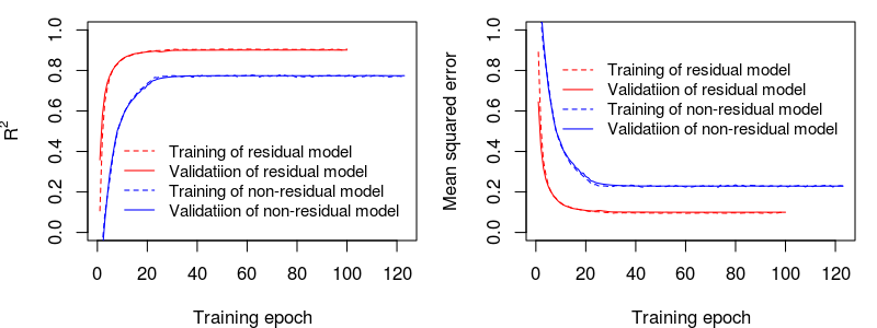
The comparison of the independent test for residual and non-residual models: performance (R2 and RMSE)
## [1] "non residual model r2: 0.78, rmse: 150.17"
## [1] "residual model r2: 0.91, rmse: 98.37"
## [1] "Residual model improved R2 by 12.48%, compared with non-residual model"
## [1] "Residual model decreased rmse by -51.8, compared with non-residual model"
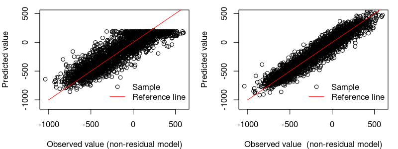
The scatter comparison of residual vs. non-residual models for the independent test:
### Example 2: Spatiotemporal Estimation of PM<sub>2.5</sub>
This dataset is the real dataset of the 2015 PM<sub>2.5</sub> and the relevant covariates for the Beijing-Tianjin-Tangshan area. Due to data security reason, it has been added with small Gaussian noise.
<img align="center" src="https://raw.githubusercontent.com/lspatial/baggingrnet/master/figs/studyregion.png" style="zoom:65%" hspace="2"/>
###### 1) Load input data:
Here the PM<sub>2.5</sub> dataset is used to test the proposed methods.
``` python
from baggingrnet.data import data
pm25_train=data('pm2.5_train')
pm25_train['gindex']=np.array([i for i in range(pm25_train.shape[0])])
```
<table>
<thead>
<tr>
<th style="text-align:left;">
</th>
<th style="text-align:left;">
sites
</th>
<th style="text-align:left;">
site\_name
</th>
<th style="text-align:left;">
city
</th>
<th style="text-align:right;">
lon
</th>
<th style="text-align:right;">
lat
</th>
<th style="text-align:right;">
pm25\_davg
</th>
<th style="text-align:right;">
ele
</th>
<th style="text-align:right;">
prs
</th>
<th style="text-align:right;">
tem
</th>
<th style="text-align:right;">
rhu
</th>
<th style="text-align:right;">
win
</th>
<th style="text-align:right;">
aod
</th>
</tr>
</thead>
<tbody>
<tr>
<td style="text-align:left;">
23123
</td>
<td style="text-align:left;">
1010A
</td>
<td style="text-align:left;">
昌平镇
</td>
<td style="text-align:left;">
北京
</td>
<td style="text-align:right;">
116.2300
</td>
<td style="text-align:right;">
40.1952
</td>
<td style="text-align:right;">
6.80000
</td>
<td style="text-align:right;">
57.0
</td>
<td style="text-align:right;">
1007.709
</td>
<td style="text-align:right;">
20.0859852
</td>
<td style="text-align:right;">
0.7609952
</td>
<td style="text-align:right;">
17.39427
</td>
<td style="text-align:right;">
0.2877372
</td>
</tr>
<tr>
<td style="text-align:left;">
1339
</td>
<td style="text-align:left;">
1014A
</td>
<td style="text-align:left;">
南口路
</td>
<td style="text-align:left;">
天津
</td>
<td style="text-align:right;">
117.1930
</td>
<td style="text-align:right;">
39.1730
</td>
<td style="text-align:right;">
84.59091
</td>
<td style="text-align:right;">
8.5
</td>
<td style="text-align:right;">
1021.859
</td>
<td style="text-align:right;">
-0.2894622
</td>
<td style="text-align:right;">
0.6565141
</td>
<td style="text-align:right;">
40.61296
</td>
<td style="text-align:right;">
0.2245625
</td>
</tr>
<tr>
<td style="text-align:left;">
11843
</td>
<td style="text-align:left;">
1062A
</td>
<td style="text-align:left;">
铁路
</td>
<td style="text-align:left;">
承德
</td>
<td style="text-align:right;">
117.9664
</td>
<td style="text-align:right;">
40.9161
</td>
<td style="text-align:right;">
21.27273
</td>
<td style="text-align:right;">
362.0
</td>
<td style="text-align:right;">
969.876
</td>
<td style="text-align:right;">
15.3092365
</td>
<td style="text-align:right;">
0.5288071
</td>
<td style="text-align:right;">
16.61683
</td>
<td style="text-align:right;">
0.4272831
</td>
</tr>
<tr>
<td style="text-align:left;">
9373
</td>
<td style="text-align:left;">
榆垡
</td>
<td style="text-align:left;">
京南榆垡,京南区域点
</td>
<td style="text-align:left;">
北京
</td>
<td style="text-align:right;">
116.3000
</td>
<td style="text-align:right;">
39.5200
</td>
<td style="text-align:right;">
12.08696
</td>
<td style="text-align:right;">
18.0
</td>
<td style="text-align:right;">
1013.116
</td>
<td style="text-align:right;">
14.0085974
</td>
<td style="text-align:right;">
0.8100768
</td>
<td style="text-align:right;">
39.46079
</td>
<td style="text-align:right;">
0.5075859
</td>
</tr>
<tr>
<td style="text-align:left;">
19596
</td>
<td style="text-align:left;">
1069A
</td>
<td style="text-align:left;">
环境监测监理中心
</td>
<td style="text-align:left;">
廊坊
</td>
<td style="text-align:right;">
116.7150
</td>
<td style="text-align:right;">
39.5571
</td>
<td style="text-align:right;">
64.20833
</td>
<td style="text-align:right;">
35.0
</td>
<td style="text-align:right;">
1005.249
</td>
<td style="text-align:right;">
24.4960499
</td>
<td style="text-align:right;">
0.8604047
</td>
<td style="text-align:right;">
14.01048
</td>
<td style="text-align:right;">
1.5149391
</td>
</tr>
</tbody>
</table>
###### 2) Set bagging path, list of predictor names, get the bagging class instance and input data:
``` python
from baggingrnet.model.bagging import multBagging
import random as r
feasList = ['lat', 'lon', 'ele', 'prs', 'tem', 'rhu', 'win', 'pblh_re', 'pre_re', 'o3_re', 'aod', 'merra2_re', 'haod',
'shaod', 'jd','lat2','lon2','latlon']
target='pm25_avg_log'
bagpath='/tmp/baggingpm25_2/res'
chkpath(bagpath)
mbag=multBagging(bagpath)
```
## initializing ...
``` python
mbag.getInputSample(pm25_train, feasList,None,'gindex',target)
```
## (29475, 31)
###### 3) Define the arguments of multiple models (here 100 models) and append them to the list of modeling duties:
``` python
import random as r
for i in range(1,81):
name = str(i)
nodes = [128 + r.randint(-5,5),128+ r.randint(-5,5),96,64,32,12]
minibatch = 2560+r.randint(-5,5)
isresidual = False
nepoch = 120
sampling_fea = False
noutput = 1
islog=True
mbag.addTask(name,noutput,sampling_fea, nepoch, nodes, minibatch, isresidual,islog)
```
###### 4) Initiate the training:
Initiate the parallel programs using 10 cores
``` python
mbag.startMProcess(10)
```
###### 5) Prediction using the trained models and optional evaluation of the trained model:
``` python
from baggingrnet.model.baggingpre import ensPrediction
prepath="/tmp/baggingpm25_2p/res"
chkpath(prepath)
mbagpre=ensPrediction(bagpath,prepath)
mbagpre.getInputSample(pm25_test, feasList,'gindex')
mbagpre.startMProcess(10)
mbagpre.aggPredict(isval=True,tfld='pm25_davg')
```
Finally, the following results were obtaned.
The results are shown as the following:
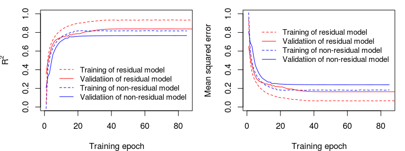
###### 1) Typical learning curves of non-residual vs. residual models are shown as the following:
###### 2) Mean performance (R2 and RMSE) of the predictions of multiple non-residual vs residual models for the independent dataset :
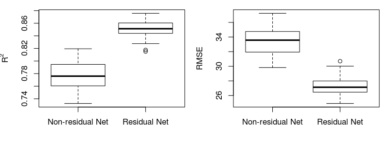
###### 3) Performance (R2 and RMSE) of the ensembled predictions based on multiple models for the independent dataset:
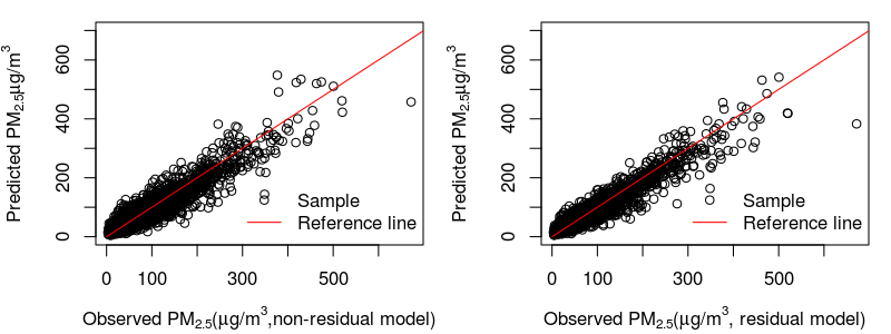
## [1] "non residual model r2: 0.88, rmse: 23.55"
## [1] "residual model r2: 0.91, rmse: 20.35"
## [1] "Residual model improved R2 by 2.97%, compared with non-residual model"
## [1] "Residual model decreased rmse by -3.2, compared with non-residual model"
###### 4) Scatter plots for the ensemble predictions of non-residual vs residual models:
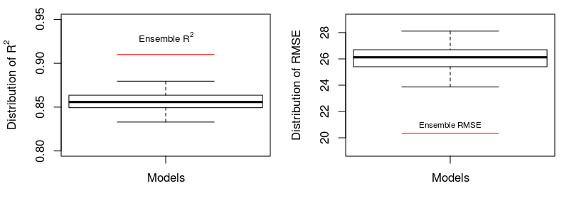
###### 5) Comparison of ensemble predictions vs. predictions of single models:
Statistics of the performance for the predictions of multiple models and ensemble predictions are made. The following shows R<sup>2</sup> and RMSE, barplots and scatter plots.
Performance digits:
## [1] "Ensemble predictions: R2=0.91, RMSE=20.35"
## [1] "Mean performance of predictions of multiple single models: R2=0.86, RMSE=26.07"
## [1] "Ensemble predictions averagely improved the single predictions by 6% for R2, and reduced -5.72ug/m3 for RMSE"
The boxplot shows considerable improvement by bagging (6% in R<sup>2</sup> and -5.72 *μ*g/m<sup>3</sup>), in comparison with single models.
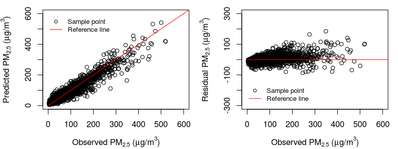
The following shows the scatter plots of observed PM<sub>2.5</sub> vs. ensemble predictions/residuals:
### Contact
For this library and its relevant complete applications, welcome to contact Dr. Lianfa Li. Email: <lspatial@gmail.com> or <lilf@lreis.ac.cn>


