MagnetiCalc
===========
[](https://pypi.org/project/MagnetiCalc/)
[](https://opensource.org/licenses/ISC)
[](https://www.paypal.com/cgi-bin/webscr?cmd=_s-xclick&hosted_button_id=TN6YTPVX36YHA&source=url)
[](https://shredengineer.github.io/MagnetiCalc/)
🍀 [Always looking for beta testers!](#contribute)
**What does MagnetiCalc do?**
MagnetiCalc calculates the static magnetic flux density, vector potential, energy, self-inductance
and magnetic dipole moment of arbitrary coils. Inside an OpenGL-accelerated GUI, the magnetic flux density
(<img src="https://render.githubusercontent.com/render/math?math=\mathbf{B}" alt="B">-field,
in units of <i>Tesla</i>)
or the magnetic vector potential
(<img src="https://render.githubusercontent.com/render/math?math=\mathbf{A}" alt="A">-field,
in units of <i>Tesla-meter</i>)
is displayed in interactive 3D, using multiple metrics for highlighting the field properties.
<i>Experimental feature:</i> To calculate the energy and self-inductance of permeable (i.e. ferrous) materials,
different core media can be modeled as regions of variable relative permeability;
however, core saturation is currently not modeled, resulting in excessive flux density values.
**Who needs MagnetiCalc?**
MagnetiCalc does its job for hobbyists, students, engineers and researchers of magnetic phenomena.
I designed MagnetiCalc from scratch, because I didn't want to mess around
with expensive and/or overly complex simulation software
whenever I needed to solve a magnetostatic problem.
**How does it work?**
The <img src="https://render.githubusercontent.com/render/math?math=\mathbf{B}" alt="B">-field calculation
is implemented using the Biot-Savart law [**1**], employing multiprocessing techniques;
MagnetiCalc uses just-in-time compilation ([JIT](https://numba.pydata.org/))
and, if available, GPU-acceleration ([CUDA](https://numba.pydata.org/numba-doc/dev/cuda/overview.html))
to achieve high-performance calculations.
Additionally, the use of easily constrainable "sampling volumes" allows for selective calculation over
grids of arbitrary shape and arbitrary relative permeabilities
<img src="https://render.githubusercontent.com/render/math?math=\mu_r(\mathbf{x})" alt="µ_r(x)">
(<i>experimental</i>).
The shape of any wire is modeled as a 3D piecewise linear curve.
Arbitrary loops of wire are sliced into differential current elements
(<img src="https://render.githubusercontent.com/render/math?math=\mathbf{\ell}" alt="l">),
each of which contributes to the total resulting field
(<img src="https://render.githubusercontent.com/render/math?math=\mathbf{A}" alt="A">,
<img src="https://render.githubusercontent.com/render/math?math=\mathbf{B}" alt="B">)
at some fixed 3D grid point (<img src="https://render.githubusercontent.com/render/math?math=\mathbf{x}" alt="x">),
summing over the positions of all current elements
(<img src="https://render.githubusercontent.com/render/math?math=\mathbf{x^'}" alt="x'">):
<img src="https://render.githubusercontent.com/render/math?math=\mathbf{A}(\mathbf{x})=I \cdot \frac{\mu_0}{4 \pi} \cdot \displaystyle \sum_\mathbf{x^'} \mu_r(\mathbf{x}) \cdot \frac{\mathbf{\ell}(\mathbf{x^')}}{\mid \mathbf{x} - \mathbf{x^'} \mid}"><br>
<img src="https://render.githubusercontent.com/render/math?math=\mathbf{B}(\mathbf{x})=I \cdot \frac{\mu_0}{4 \pi} \cdot \displaystyle \sum_\mathbf{x^'} \mu_r(\mathbf{x}) \cdot \frac{\mathbf{\ell}(\mathbf{x^'}) \times (\mathbf{x} - \mathbf{x^'})}{\mid \mathbf{x} - \mathbf{x^'} \mid}"><br>
At each grid point, the field magnitude (or field angle in some plane) is displayed
using colored arrows and/or dots;
field color and alpha transparency are individually mapped using one of the various
[available metrics](#appendix-metrics).
The coil's energy <img src="https://render.githubusercontent.com/render/math?math=E" alt="E"> [**2**]
and self-inductance <img src="https://render.githubusercontent.com/render/math?math=L" alt="L"> [**3**]
are calculated by summing the squared
<img src="https://render.githubusercontent.com/render/math?math=\mathbf{B}" alt="B">-field
over the entire sampling volume;
ensure that the sampling volume encloses a large, non-singular portion of the field:
<img src="https://render.githubusercontent.com/render/math?math=E=\frac{1}{\mu_0} \cdot \displaystyle \sum_\mathbf{x} \frac{\mathbf{B}(\mathbf{x}) \cdot \mathbf{B}(\mathbf{x})}{\mu_r(\mathbf{x})}"><br>
<img src="https://render.githubusercontent.com/render/math?math=L=\frac{1}{\I^2} \cdot E"><br>
Additionally, the scalar magnetic dipole moment
<img src="https://render.githubusercontent.com/render/math?math=m" alt="m"> [**4**]
is calculated by summing over all current elements:
<img src="https://render.githubusercontent.com/render/math?math=m=\Bigl| I \cdot \frac{1}{2} \cdot \displaystyle \sum_\mathbf{x^'} \mathbf{x^'} \times \mathbf{\ell}(\mathbf{x^'}) \Bigr|"><br>
***References***
[**1**]: Jackson, Klassische Elektrodynamik, 5. Auflage, S. 204, (5.4).<br>
[**2**]: Kraus, Electromagnetics, 4th Edition, p. 269, 6-9-1.<br>
[**3**]: Jackson, Klassische Elektrodynamik, 5. Auflage, S. 252, (5.157).<br>
[**4**]: Jackson, Klassische Elektrodynamik, 5. Auflage, S. 216, (5.54).
Screenshot
----------
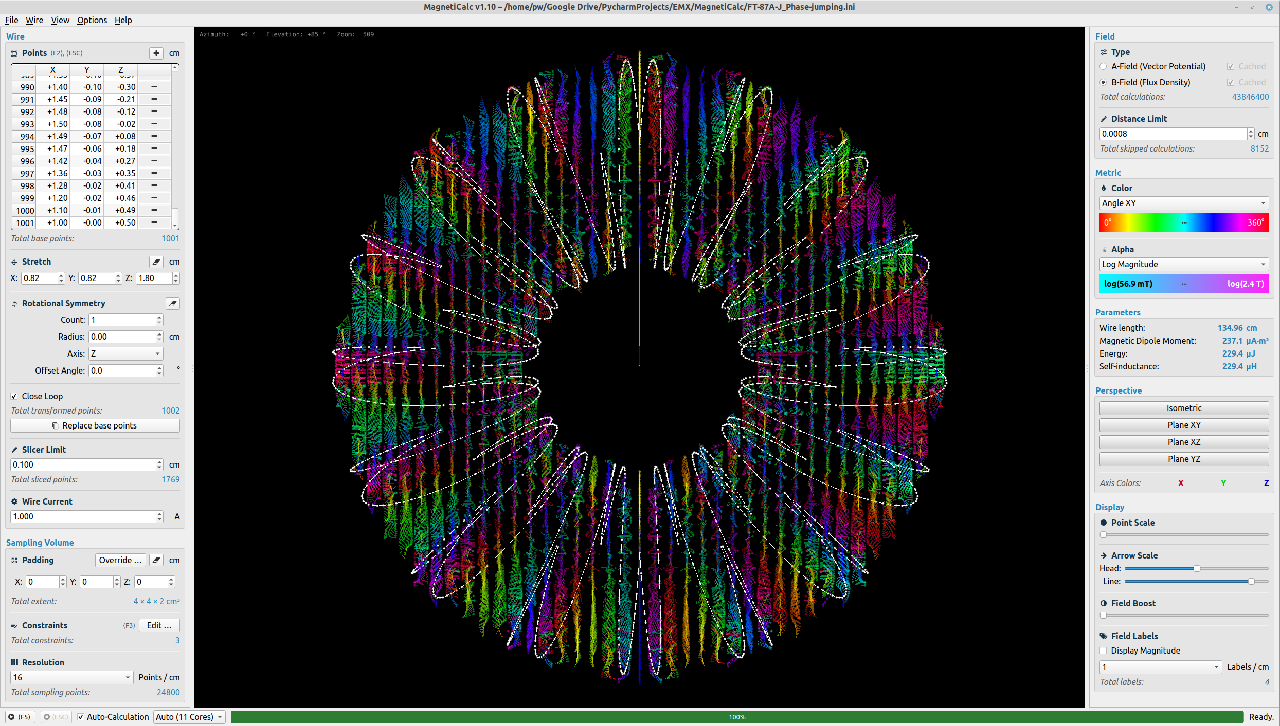
(Screenshot taken from the latest GitHub release.)
Examples
--------
Some example projects can be found in the `examples/` folder.
If you feel like your project should also be included as an example, you are welcome to file an [issue](https://github.com/shredEngineer/MagnetiCalc/issues)!
Installation
------------
If you have trouble installing MagnetiCalc,
make sure to file an [issue](https://github.com/shredEngineer/MagnetiCalc/issues)
so I can help you get it up and running!
Requirements:
* Python 3.6+
Tested with:
* Python 3.7 in Linux Mint 19.3
* Python 3.8 in Ubuntu 20.04
* Python 3.8.2 in macOS 11.6 (M1)
* Python 3.8.10 in Windows 10 (21H2)
* Python 3.10.5 in Ubuntu 20.04
### Prerequisites
On some systems, it may be necessary to upgrade pip first:
`python3 -m pip install pip --upgrade`
*Note:* Windows users need to type `python` instead of `python3`
#### Linux
The following dependencies must be installed first (Ubuntu 20.04):
```shell
sudo apt install python3-dev
sudo apt install libxcb-xinerama0 --reinstall
```
#### Windows
It is recommended to install [Python 3.8.10](https://www.python.org/downloads/release/python-3810/).
Installation will currently fail for Python 3.9+ due to missing dependencies.
On some systems, it may be necessary to install the latest
[Microsoft Visual C++ Redistributable](https://docs.microsoft.com/en-us/cpp/windows/latest-supported-vc-redist?view=msvc-170)
first.
#### macOS (M1)
On Apple Silicon,
[Open Using Rosetta](https://www.courier.com/blog/tips-and-tricks-to-setup-your-apple-m1-for-development/)
must be enabled for the Terminal app before installing (upgrading) and starting MagnetiCalc.
### Option A: Automatic install via pip
This will install (upgrade) MagnetiCalc (and its dependencies) to the user site-packages directory and start it.
[](https://pypi.org/project/MagnetiCalc/)
#### Linux & macOS (Intel)
```shell
python3 -m pip install magneticalc --upgrade
python3 -m magneticalc
```
#### Windows
```shell
python -m pip install --upgrade magneticalc
python -m magneticalc
```
#### macOS (M1)
*Note:* On Apple Silicon, JIT must be disabled due to incomplete support, resulting in slow calculations.
```shell
python3 -m pip install magneticalc --upgrade
export NUMBA_DISABLE_JIT=1 && python3 -m magneticalc
```
#### Juptyer Notebook & Jupyter Lab
From within a [Jupyter](https://jupyter.org/) Notebook, MagnetiCalc can be installed (upgraded) and run like this:
```python
import sys
!{sys.executable} -m pip install magneticalc --upgrade
!{sys.executable} -m magneticalc
```
### Option B: Manual download
*Note:* Windows users need to type `python` instead of `python3`.
Install (upgrade) all dependencies to the user site-packages directory:
```shell
python3 -m pip install numpy numba scipy PyQt5 vispy qtawesome sty si-prefix h5py --upgrade
```
Use [Git](https://git-scm.com/) to clone the latest version of MagnetiCalc from GitHub:
```shell
git clone https://github.com/shredEngineer/MagnetiCalc
```
Enter the cloned directory and start MagnetiCalc:
```shell
cd MagnetiCalc
python3 -m magneticalc
```
### Enabling CUDA Support
Tested in Ubuntu 20.04, using the NVIDIA CUDA 10.1 driver and NVIDIA GeForce GTX 1650 GPU.
Please refer to the
[Numba Installation Guide](https://numba.pydata.org/numba-doc/latest/user/installing.html)
which includes the steps necessary to get CUDA up and running.
License
-------
Copyright © 2020–2022, Paul Wilhelm, M. Sc. <[anfrage@paulwilhelm.de](mailto:anfrage@paulwilhelm.de)>
<b>ISC License</b>
Permission to use, copy, modify, and/or distribute this software for any
purpose with or without fee is hereby granted, provided that the above
copyright notice and this permission notice appear in all copies.
THE SOFTWARE IS PROVIDED "AS IS" AND THE AUTHOR DISCLAIMS ALL WARRANTIES
WITH REGARD TO THIS SOFTWARE INCLUDING ALL IMPLIED WARRANTIES OF
MERCHANTABILITY AND FITNESS. IN NO EVENT SHALL THE AUTHOR BE LIABLE FOR
ANY SPECIAL, DIRECT, INDIRECT, OR CONSEQUENTIAL DAMAGES OR ANY DAMAGES
WHATSOEVER RESULTING FROM LOSS OF USE, DATA OR PROFITS, WHETHER IN AN
ACTION OF CONTRACT, NEGLIGENCE OR OTHER TORTIOUS ACTION, ARISING OUT OF
OR IN CONNECTION WITH THE USE OR PERFORMANCE OF THIS SOFTWARE.
[](https://opensource.org/licenses/ISC)
Contribute
----------
**You** are invited to contribute to MagnetiCalc!
General feedback, Issues and Pull Requests are always welcome.
If this software has been helpful to you in some way or another, please let me and others know!
[](https://www.paypal.com/cgi-bin/webscr?cmd=_s-xclick&hosted_button_id=TN6YTPVX36YHA&source=url)
Documentation
-------------
The documentation for MagnetiCalc is auto-generated from docstrings in the Python code.
[](https://shredengineer.github.io/MagnetiCalc/)
### Debugging
If desired, MagnetiCalc can be quite verbose about everything it is doing in the terminal:
* Some modules are blacklisted in [`Debug.py`](magneticalc/Debug.py), but this can easily be changed.
* Some modules also provide their own debug switches to increase the level of detail.
Data Import/Export and Python API
---------------------------------
### GUI
MagnetiCalc allows the following data to be imported/exported using the GUI:
* Import/export wire points from/to TXT file.
* Export <img src="https://render.githubusercontent.com/render/math?math=\mathbf{A}" alt="A">-/<img src="https://render.githubusercontent.com/render/math?math=\mathbf{B}" alt="B">-fields,
wire points and wire current to an [HDF5](https://www.h5py.org/) container for use in post-processing.<br>
*Note:* You could use [Panoply](https://www.giss.nasa.gov/tools/panoply/download/) to open HDF5 files.
(The "official" [HDFView](https://www.hdfgroup.org/downloads/hdfview/) software didn't work for me.)
### API
The [`API`](magneticalc/API.py) class
([documentation](https://shredengineer.github.io/MagnetiCalc/magneticalc.API.API.html))
provides basic functions for importing/exporting data programmatically.
#### Example: Wire Export
Generate a wire shape using [NumPy](https://numpy.org/) and export it to a TXT file:
```python
from magneticalc import API
import numpy as np
wire = [
(np.cos(a), np.sin(a), np.sin(16 * a) / 5)
for a in np.linspace(0, 2 * np.pi, 200)
]
API.export_wire("Custom Wire.txt", wire)
```
#### Example: Field Import
Import an HDF5 file containing an
<img src="https://render.githubusercontent.com/render/math?math=\mathbf{A}" alt="A">-field
and plot it using [Matplotlib](https://matplotlib.org/stable/users/index.html):
```python
from magneticalc import API
import matplotlib.pyplot as plt
data = API.import_hdf5("examples/Custom Export.hdf5")
axes = data.get_axes()
a_field = data.get_a_field()
ax = plt.figure(figsize=(5, 5), dpi=150).add_subplot(projection="3d")
ax.quiver(*axes, *a_field, length=1e5, normalize=False, linewidth=.5)
plt.show()
```
The imported data is wrapped in a [`MagnetiCalc_Data`](magneticalc/MagnetiCalc_Data.py) object
([documentation](https://shredengineer.github.io/MagnetiCalc/magneticalc.MagnetiCalc_Data.MagnetiCalc_Data.html))
which provides convenience functions for accessing, transforming and reshaping the data:
| Method | Description |
|----------------------------------------------------------|------------------------------------------------------------------------------------------------------------------------------------------------------------------------------------------------------------------------------------------------------------------|
| `.get_wire_list()` | Returns a list of all 3D points of the wire. |
| `.get_wire()` | Returns the raveled wire points as three arrays. |
| `.get_current()` | Returns the wire current. |
| `.get_dimension()` | Returns the sampling volume dimension as a 3-tuple. |
| `.get_axes_list()` | Returns a list of all 3D points of the sampling volume. |
| `.get_axes()` | Returns the raveled sampling volume coordinates as three arrays. |
| `.get_axes(reduce=True)` | Returns the axis ticks of the sampling volume. |
| `.get_a_field_list()`<br>`.get_b_field_list()` | Returns a list of all 3D vectors of the <img src="https://render.githubusercontent.com/render/math?math=\mathbf{A}" alt="A">- or <img src="https://render.githubusercontent.com/render/math?math=\mathbf{B}" alt="B">-field. |
| `.get_a_field()`<br>`.get_b_field()` | Returns the raveled <img src="https://render.githubusercontent.com/render/math?math=\mathbf{A}" alt="A">- or <img src="https://render.githubusercontent.com/render/math?math=\mathbf{B}" alt="B">-field coordinates as three arrays. |
| `.get_a_field(as_3d=True)`<br>`.get_b_field(as_3d=True)` | Returns a 3D field for each component of the <img src="https://render.githubusercontent.com/render/math?math=\mathbf{A}" alt="A">- or <img src="https://render.githubusercontent.com/render/math?math=\mathbf{B}" alt="B">-field, indexed over the reduced axes. |
ToDo
----
**Functional**
* Add a histogram for every metric.
* Add an overlay for vector metrics, like gradient or curvature
(derived from the fundamental
<img src="https://render.githubusercontent.com/render/math?math=\mathbf{A}" alt="A">- and
<img src="https://render.githubusercontent.com/render/math?math=\mathbf{B}" alt="B">-fields).
* Add a list of objects, for wires and permeability groups (constraints),
with a transformation pipeline for each object;
move the `Wire` widget to a dedicated dialog window instead.
(Add support for multiple wires, study mutual induction.)
* Interactively display superposition of fields with varying currents.
* Add (cross-)stress scalar metric: Ratio of absolute flux density contribution to actual flux density at every point.
* Highlight permeability groups with
<img src="https://render.githubusercontent.com/render/math?math=\mu_r \neq 0"> in the 3D view.
* Add support for multiple current values and animate the resulting fields.
* Add support for modeling of core material saturation and hysteresis effects.
* Provide a means to emulate permanent magnets.
**Usability**
* Move variations of each wire preset (e.g. the number of turns) into an individual sub-menu;
alternatively, provide a dialog for parametric generation.
* Add stationary coordinate system and ruler in the bottom left corner.
* Add support for selective display over a portion of the metric range,
enabling a kind of iso-contour display.
**Known Bugs**
* Fix issue where the points of a sampling volume with *fractional* resolution
are not always spaced equidistantly for some sampling volume dimensions.
* Fix calculation of divergence right at the sampling volume boundary.
* Fix missing scaling of VisPy markers when zooming.
* Fix unnecessary shading of VisPy markers.
**Performance**
* Parallelize sampling volume calculation which is currently slow.
**Code Quality**
* Add unit tests.
Video
-----
A very short demo of MagnetiCalc in action:
[](https://www.youtube.com/watch?v=d3QKdYfOuvQ)
Links
-----
There is also a short article about MagnetiCalc on my personal website:
[paulwilhelm.de/magneticalc](https://paulwilhelm.de/magneticalc/)
*Appendix:* Metrics
-------------------
| Metric | Symbol | Description |
|----------------------|--------------------------------------------------------------------------------------------------------------|---------------------------------------|
| ``Magnitude`` | <img src="https://render.githubusercontent.com/render/math?math=\mid\vec{B}\mid"> | Magnitude in space |
| ``Magnitude X`` | <img src="https://render.githubusercontent.com/render/math?math=\mid\vec{B}_{X}\mid"> | Magnitude in X-direction |
| ``Magnitude Y`` | <img src="https://render.githubusercontent.com/render/math?math=\mid\vec{B}_{Y}\mid"> | Magnitude in Y-direction |
| ``Magnitude Z`` | <img src="https://render.githubusercontent.com/render/math?math=\mid\vec{B}_{Z}\mid"> | Magnitude in Z-direction |
| ``Magnitude XY`` | <img src="https://render.githubusercontent.com/render/math?math=\mid\vec{B}_{XY}\mid"> | Magnitude in XY-plane |
| ``Magnitude XZ`` | <img src="https://render.githubusercontent.com/render/math?math=\mid\vec{B}_{XZ}\mid"> | Magnitude in XZ-plane |
| ``Magnitude YZ`` | <img src="https://render.githubusercontent.com/render/math?math=\mid\vec{B}_{YZ}\mid"> | Magnitude in YZ-plane |
| ``Divergence`` | <img src="https://render.githubusercontent.com/render/math?math=\nabla\cdot\vec{B}"> | Divergence |
| ``Divergence +`` | <img src="https://render.githubusercontent.com/render/math?math=%2b\{\nabla\cdot\vec{B}\}_{>0}"> | Positive Divergence |
| ``Divergence –`` | <img src="https://render.githubusercontent.com/render/math?math=-\{\nabla\cdot\vec{B}\}_{<0}"> | Negative Divergence |
| ``Log Magnitude`` | <img src="https://render.githubusercontent.com/render/math?math=\log_{10} \mid\vec{B}\mid"> | Logarithmic Magnitude in space |
| ``Log Magnitude X`` | <img src="https://render.githubusercontent.com/render/math?math=\log_{10} \mid\vec{B_X}\mid"> | Logarithmic Magnitude in X-direction |
| ``Log Magnitude Y`` | <img src="https://render.githubusercontent.com/render/math?math=\log_{10} \mid\vec{B_Y}\mid"> | Logarithmic Magnitude in Y-direction |
| ``Log Magnitude Z`` | <img src="https://render.githubusercontent.com/render/math?math=\log_{10} \mid\vec{B_Z}\mid"> | Logarithmic Magnitude in Z-direction |
| ``Log Magnitude XY`` | <img src="https://render.githubusercontent.com/render/math?math=\log_{10} \mid\vec{B}_{XY}\mid"> | Logarithmic Magnitude in XY-plane |
| ``Log Magnitude XZ`` | <img src="https://render.githubusercontent.com/render/math?math=\log_{10} \mid\vec{B}_{XZ}\mid"> | Logarithmic Magnitude in XZ-plane |
| ``Log Magnitude YZ`` | <img src="https://render.githubusercontent.com/render/math?math=\log_{10} \mid\vec{B}_{YZ}\mid"> | Logarithmic Magnitude in YZ-plane |
| ``Log Divergence`` | <img src="https://render.githubusercontent.com/render/math?math=\log_{10} \ \ \nabla\cdot\vec{B}"> | Logarithmic Divergence |
| ``Log Divergence +`` | <img src="https://render.githubusercontent.com/render/math?math=\log_{10} \ %2b\{\nabla\cdot\vec{B}\}_{>0}"> | Positive Logarithmic Divergence |
| ``Log Divergence –`` | <img src="https://render.githubusercontent.com/render/math?math=\log_{10} \ -\{\nabla\cdot\vec{B}\}_{<0}"> | Negative Logarithmic Divergence |
| ``Angle XY`` | <img src="https://render.githubusercontent.com/render/math?math=\measuredangle\vec{B}_{XY}"> | Field angle in XY-plane |
| ``Angle XZ`` | <img src="https://render.githubusercontent.com/render/math?math=\measuredangle\vec{B}_{XZ}"> | Field angle in XZ-plane |
| ``Angle YZ`` | <img src="https://render.githubusercontent.com/render/math?math=\measuredangle\vec{B}_{YZ}"> | Field angle in YZ-plane |


