# Psychometric curve fitting
 [](https://sonarcloud.io/dashboard?id=garethjns_PsychometricCurveFitting)
Fitting for Psychometric curves in Python and Matlab. Supports:
- [Simple logit link function (mean and varience parameters)](https://en.wikipedia.org/wiki/Psychometric_function).
- [Wichmann and Hill 2001](http://wexler.free.fr/library/files/wichmann%20(2001)%20the%20psychometric%20function.%20i.%20fitting,%20sampling,%20and%20goodness%20of%20fit.pdf). This curve adds two additional parameters, "guess" and "lapse", which control somewhat for subject fallibility, improving the estimate of the discrimination threshold.
# Python usage
````bash
pip install fit-psyche
````
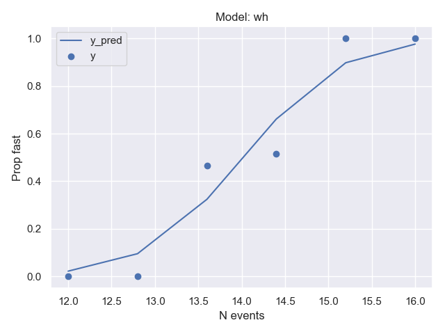
## Using the sklearn API.
````python
import numpy as np
from fit_psyche.psychometric_curve import PsychometricCurve
x = np.linspace(start=12, stop=16, num=6)
y = (x > x.mean()).astype(float)
y[2] = y[2] + np.abs(np.random.rand())
y[3] = y[3] - np.abs(np.random.rand())
pc = PsychometricCurve(model='wh').fit(x, y)
pc.plot(x, y)
print(pc.score(x, y))
print(pc.coefs_)
````
```
>>> 0.9796769364413764
>>> {'mean': 13.829364486404069,
'var': 0.9658606821413274,
'guess_rate': 0.010000000000000002,
'lapse_rate': 0.010000000000000002}
```
Assuming enough data is available, this is also compatible with CV search objects, for example:
```python
import numpy as np
from sklearn.model_selection import RandomizedSearchCV
from fit_psyche.psychometric_curve import PsychometricCurve
x = np.linspace(start=12, stop=16, num=16)
y = (x > x.mean()).astype(float)
y[2] = y[2] + np.abs(np.random.rand())
y[3] = y[3] - np.abs(np.random.rand())
grid = RandomizedSearchCV(PsychometricCurve(), n_jobs=3,
param_distributions={'model': ['wh', 'logit'],
'guess_rate_lims': [(0.01, 0.05), (0.01, 0.03), (0.03, 0.04)],
'lapse_rate_lims': [(0.01, 0.05), (0.01, 0.03), (0.03, 0.04)]})
grid.fit(x, y)
print(grid.best_estimator_.get_params())
print(grid.best_estimator_.coefs_)
```
```
>>> {'guess_rate_lims': (0.03, 0.04),
'lapse_rate_lims': (0.01, 0.05),
'mean_lims': (0, 20),
'model': 'wh',
'var_lims': (0.001, 20)}
>>> {'mean': 14.001413727640738,
'var': 0.027772082199237953,
'guess_rate': 0.030000000000000002,
'lapse_rate': 0.01000000000000001}
```
# Matlab Usage
Fitting functions can be accessed by creating a PsychFit object, or directly. See also examples in scripts/.
```MATLAB
% Make up some data
y1 = [0 0 25 25 50 50 75 75 100 100]/100;
y2 = [20 20 20 30 40 60 70 80 80 80];
y2 = (y2+rand(1,numel(y2))*5)/100;
% Create x axis
x = 0.1:0.1:1;
```
## PsychFit object
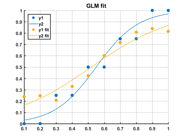
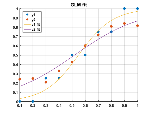
### GLM
```MATLAB
ffit1 = fitPsyche(x, y1, 'GLM');
ffit2 = fitPsyche(x, y2, 'GLM');
figure
plotPsyche(ffit1)
hold on
plotPsyche(ffit2)
legend({'y1', 'y2', 'y1 fit', 'y2 fit'}, 'Location', 'NorthWest')
title('GLM fit')
```
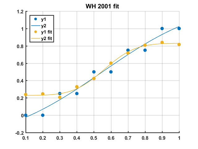
### WH2001
```MATLAB
ffit1 = fitPsyche(x, y1, 'WH');
ffit2 = fitPsyche(x, y2, 'WH');
figure
plotPsyche(ffit1)
hold on
plotPsyche(ffit2)
legend({'y1', 'y2', 'y1 fit', 'y2 fit'}, 'Location', 'NorthWest')
title('WH 2001 fit')
disp(ffit1.model)
disp(ffit2.model)
```
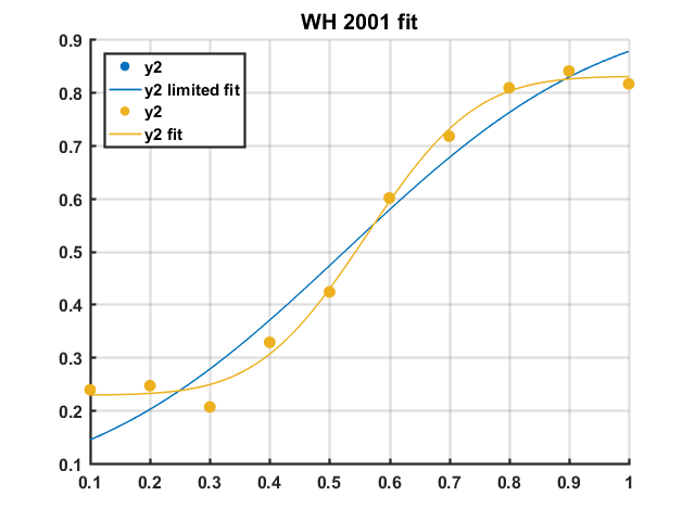
### WH2001 with limited coefficients
```MATLAB
%% Set limits for WH fit
% g (guess rate), l (lapse), u (mean, bias), v (variance, discrimination
% thresh)
% UpperLimits:
UL = [0.05, 0.05, 1, 1]; % Limit upper bound of g and l to 5%
% StartPoints:
SP = [0, 0, 0.5, 0.5];
% LowerLimits:
LL = [0.05, 0.05, 0, 0];
ffit1 = fitPsyche(x, y2, 'WH', [UL;SP;LL]);
ffit2 = fitPsyche(x, y2, 'WH');
figure
plotPsyche(ffit1)
hold on
plotPsyche(ffit2)
legend({'y2', 'y2 limited fit', 'y2', 'y2 fit'}, 'Location', 'NorthWest')
title('WH 2001 fit')
disp(ffit1.model)
disp(ffit2.model)
```
## Direct method access
### GLM
```MATLAB
%% Fit GLM - access methods directly
[coeffs1, curve1, ~] = ...
fitPsyche.fitPsycheCurveLogit(x, y1);
[coeffs2, curve2, ~] = ...
fitPsyche.fitPsycheCurveLogit(x, y2);
% Plot
figure
scatter(x', y1')
hold on
scatter(x', y2')
plot(curve1(:,1),curve1(:,2))
plot(curve2(:,1),curve2(:,2))
legend({'y1', 'y2', 'y1 fit', 'y2 fit'}, 'Location', 'NorthWest')
title('GLM fit')
```
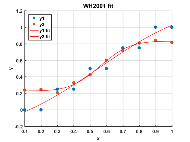
### WH2001
```MATLAB
[ffit1, curve1] = ...
fitPsyche.fitPsycheCurveWH(x, y1);
[ffit2, curve2] = ...
fitPsyche.fitPsycheCurveWH(x, y2);
% Plot
figure
scatter(x', y1')
hold on
scatter(x', y2')
plot(ffit1)
plot(ffit2)
legend({'y1', 'y2', 'y1 fit', 'y2 fit'}, 'Location', 'NorthWest')
title('WH2001 fit')
```